Analysis and prediction of Telecom user churn
- 1, Project background
- 2, Analysis purpose
- 3, Data source
- 4, Ask questions
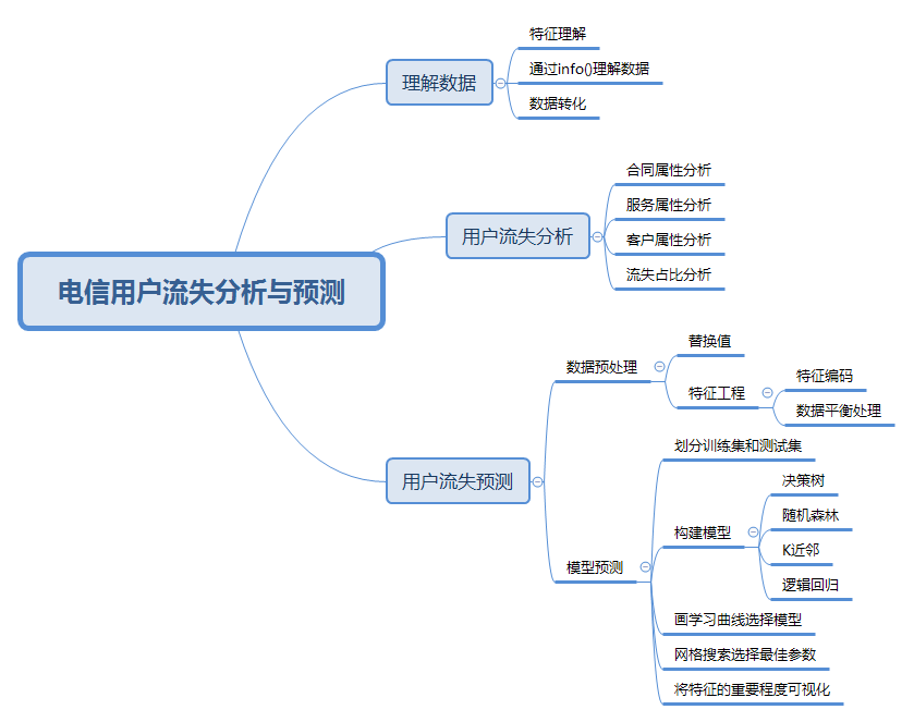
- 5, Analysis process
- 6, Understanding data
- 7, User churn analysis
- 1. Analysis of loss proportion
- 2. User attribute analysis
- 3. User attribute analysis
- 4. Contract attribute analysis
- 8, User churn forecast
- 9, Analysis suggestions
1, Project background
In recent years, both the traditional industry and the Internet industry are facing the problem of user churn. The research shows that an enterprise can lose 100 users in a week and get another user at the same time. From the perspective of the result, the performance has not been affected. In fact, the cost of publicity and promotion for these new users is much more expensive than that of maintaining the old users. From the Perspective of the return on investment, it is very uneconomical.
The importance of maintaining the old users is mainly reflected in the following four aspects:
- Retaining the old users can make the competition of the enterprise longer.
- Retaining old users will also significantly reduce costs.
- Retaining the old users will greatly benefit the development of new users. If a satisfied user leads to 8 potential businesses, at least one of them will be closed.
- Get more user share. Loyal users will be more willing to buy the enterprise's products, and their spending will be much larger than casual consumers.
2, Analysis purpose
This paper will analyze the characteristics and causes of lost users, help operators to find and improve user experience, and determine the retention target users and make plans.
3, Data source
This dataset is from Loss of kaggle telecom users data set
4, Ask questions
- Analyze the relationship between user characteristics and churn
- From the overall situation, what are the general characteristics of lost users?
- Try to find a suitable model to predict the loss of users.
- Suggestions are given to increase user viscosity and prevent loss.
5, Analysis process
6, Understanding data
1. Feature understanding
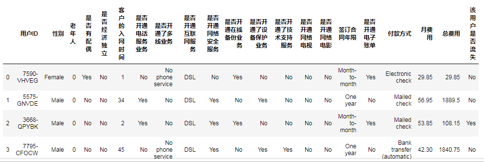
The following are the contents, types and meanings of data indicators.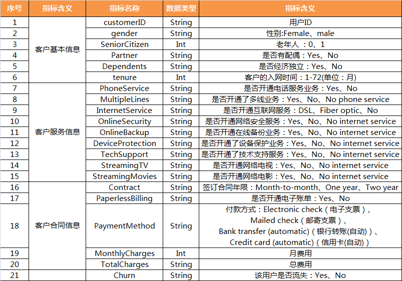
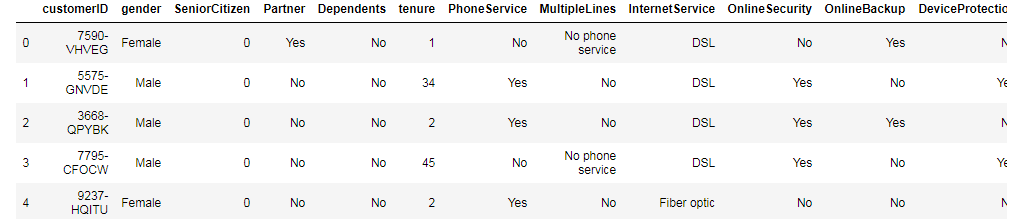
2. Import data
data=pd.read_csv('WA_Fn-UseC_-Telco-Customer-Churn.csv')
#Set show all columns
pd.set_option('display.max_columns',None)
#Set to show all rows
# pd.set_option('display.max_rows',None)
data.head()
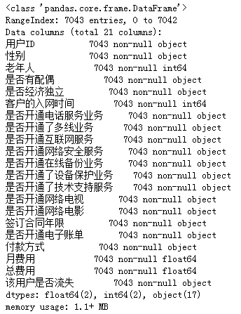
Observe and understand the data with info().
data.info()
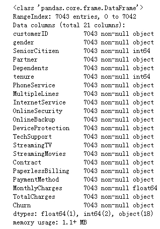
It can be seen that there are 7043 records and 21 fields in the data. The data types mainly include object string, int64 numeric type and float64 floating-point type. Where the data type of TotalCharges is string, it should be converted to floating-point type.
3. Data transformation
For ease of understanding, I changed the column name to Chinese.
data.columns=['user ID','Gender','aged' ,'Spouse or not' ,'Economic independence or not' ,'Access time of customers','Open telephone service or not' ,'Whether multi line service has been opened'
,'Whether to open Internet service' ,'Whether to open network security service','Whether to open online backup service','Whether the equipment protection business has been opened','Whether the technical support service has been opened','Whether to open network TV'
,'Open online movie or not','Years of signing the contract' ,'Open electronic bill or not','payment method','Monthly expenses','Total cost','Whether the user is lost']
data.head()
Error converting total charge to floating point type: ValueError: could not convert string to float: string cannot be converted to floating point type.
data['Total cost'].astype(float)
#Operation result:
could not convert string to float:
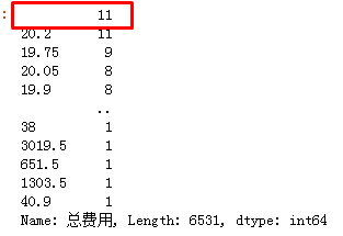
Check the data again and find the missing value.
data['Total cost'].value_counts()
Check other columns for missing values in turn.
for i in data.columns:
    test=data[i].value_counts()
    print('[{0}The number of rows is:{1}'.format(i,test.sum()))
    print('[{0}The content is:\n{1}\n'.format(i,test))
Force total charge to floating point type.
data['Total cost']=data['Total cost'].apply(pd.to_numeric, errors="coerce")
data[data['Total cost'].isnull()][['Customer access time','Total cost']]
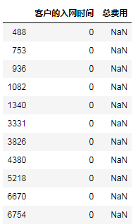
After the conversion to floating-point type, it is found that the user access time of missing value is 0. It is speculated that there is no total cost in the first month of user access. Therefore, the total cost is filled into the monthly cost, and the user's access time is changed to 1.
data['Total cost'].fillna(data[data['Total cost'].isnull()]['Monthly expenses'],axis=0,inplace=True)
data['Access time of customers'].replace(to_replace=0,value=1,inplace=True)
data.info()
Data processing completed.
7, User churn analysis
1. Analysis of loss proportion
Check the loss of users.
plt.rcParams['font.sans-serif']=['SimHei']
plt.rcParams['axes.unicode_minus']=False
plt.pie(data['Whether the user is lost'].value_counts(),labels=['Not lost','Loss'],autopct='%.2f%%',explode=(0.1,0))
plt.title('Proportion of users lost')
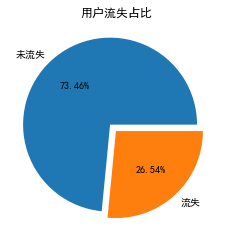
It can be seen that about one third of the users are lost.
2. User attribute analysis
def plt_bar(featrue):
    df=(data.groupby(data[featrue])['Whether the user is lost'].value_counts()/len(data)).unstack()
    df.plot(kind='bar')
    plt.title('{}Loss analysis'.format(featrue),fontsize=15)
    plt.xticks(rotation=0)
    plt.rcParams.update({'font.size': 10})
plt_bar('Gender')
plt_bar('aged')
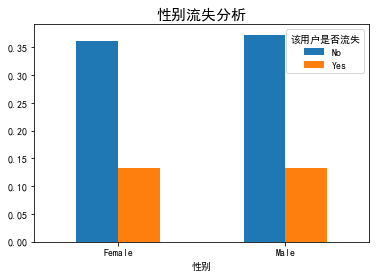
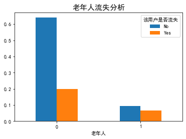
Summary:
- The loss of users has nothing to do with gender.
- The proportion of old users lost is significantly higher than that of young users.
def plt_kde(feature):
    x=data[data['Whether the user is lost']=='Yes'][feature]
    y=data[data['Whether the user is lost']=='No'][feature]
    sns.kdeplot(x,shade=True,label='Lost customers')
    sns.kdeplot(y,shade=True,label='No lost customers')
    plt.title('{}analysis'.format(feature),fontsize=15)
plt_kde('Customer access time')
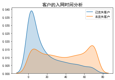
Summary:
- The shorter the user's access time, the higher the loss, in line with the general law.
- The risk of user loss is the highest in 0-20 days.
- The network access time is three months, and the loss rate is less than the on-line rate, which proves that the user's psychological stability period is generally three months.
plt_bar('Spouse or not')
plt_bar('Economic independence or not')
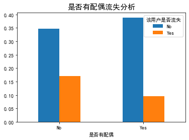
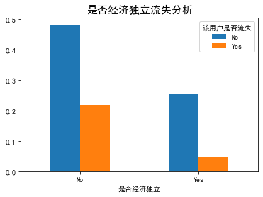
Summary:
- The loss rate of users without spouse is higher than that of users with spouse.
- The loss rate of users without economic independence is higher than that of economic independence.
3. User attribute analysis
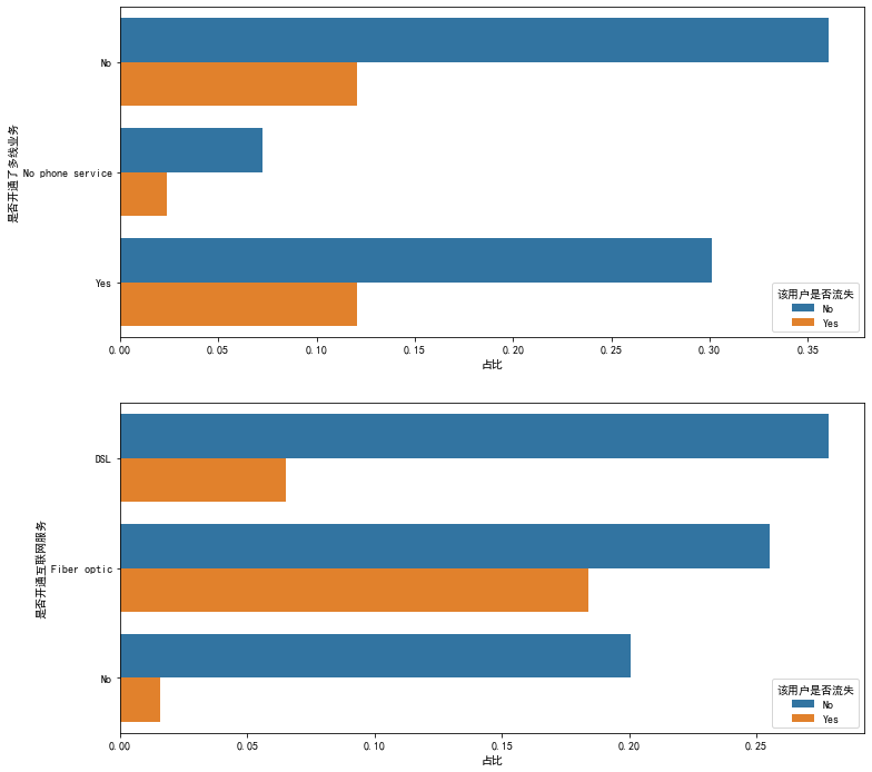
def plt_hbar(feature1,feature2):
    figure,ax=plt.subplots(2,1,figsize=(12,12))
    gp_dep=(data.groupby(feature1)['Whether the user is lost'].value_counts()/len(data)).to_frame()
    gp_dep.rename(columns={"Whether the user is lost":'Proportion'} , inplace=True)
    gp_dep.reset_index(inplace=True)
    sns.barplot(x='Proportion', hue='Whether the user is lost',y=feature1, data=gp_dep,ax=ax[0])

    gp=(data.groupby(feature2)['Whether the user is lost'].value_counts()/len(data)).to_frame()
    gp.rename(columns={"Whether the user is lost":'Proportion'} , inplace=True)
    gp.reset_index(inplace=True)
    sns.barplot(x='Proportion', hue='Whether the user is lost',y=feature2, data=gp,ax=ax[1])
plt_hbar("Whether multi line service has been opened","Whether to open Internet service")
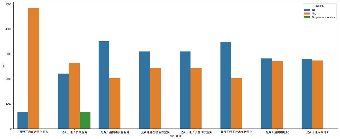
df1=pd.melt(data[data['Whether to open Internet service']!='No'][['Open telephone service or not','Whether multi line service has been opened','Whether to open network security service'
 ,'Whether to open online backup service','Whether the equipment protection business has been opened','Whether the technical support service has been opened'
,'Whether to open network TV','Open online movie or not']],value_name='Service available')
plt.figure(figsize=(20, 8))
sns.countplot(data=df1,x='variable',hue='Service available')
df2=pd.melt(data[(data['Whether to open Internet service']!='No')& (data['Whether the user is lost']=='Yes')][['Open telephone service or not','Whether multi line service has been opened','Whether to open network security service'
 ,'Whether to open online backup service','Whether the equipment protection business has been opened','Whether the technical support service has been opened'
,'Whether to open network TV','Open online movie or not']])
figure,ax=plt.subplots(figsize=(16,8))
sns.countplot(x='variable',hue='value',data=df2)
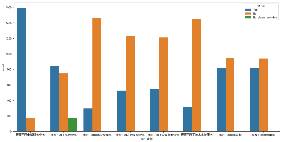
Summary:
- Telephone service has little impact on the overall loss.
- The loss of single fiber users is relatively high.
- The loss rate of optical fiber users with security, backup, protection and technical support services is low
- The loss rate of additional network TV and film services for optical fiber users is relatively high.
4. Contract attribute analysis
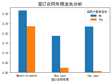
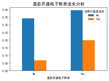
plt_bar('Years of signing the contract')
plt_bar('Open electronic bill or not')
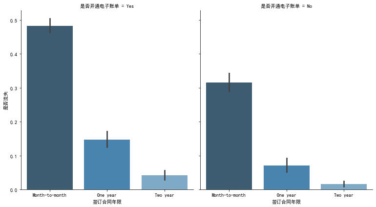
data['Loss or not']=data['Whether the user is lost'].replace('No',0).replace('Yes',1)
g = sns.FacetGrid(data, col="Open electronic bill or not", height=6, aspect=.9)
ax = g.map(sns.barplot, "Years of signing the contract","Loss or not",palette = "Blues_d"
           , order= ['Month-to-month', 'One year', 'Two year'])
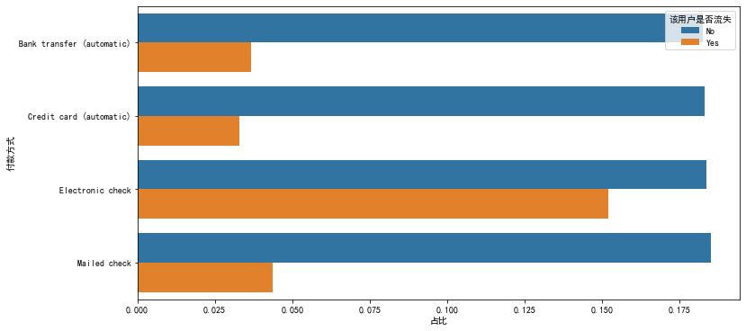
figure,ax=plt.subplots(figsize=(12,6))
gp_dep=(data.groupby('payment method')['Whether the user is lost'].value_counts()/len(data)).to_frame()
gp_dep.rename(columns={"Whether the user is lost":'Proportion'} , inplace=True)
gp_dep.reset_index(inplace=True)
sns.barplot(x='Proportion', hue='Whether the user is lost',y='payment method', data=gp_dep)
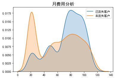
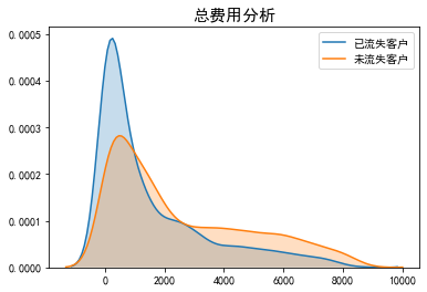
plt_kde('Monthly expenses')
plt_kde('Total cost')
- The churn rate of users who have signed the contract years: sign by month > sign by one year > sign by two years, proving that the long-term contract can retain users.
- The high loss rate of users who open electronic bills is due to the high proportion of users who sign contracts on a monthly basis, low user stickiness and easy loss.
- The loss rate of users using electronic check is the highest. It is speculated that the use experience of this method is general.
- The monthly consumption amount is about 70-110 with a high user churn rate.
- In the long run, the higher the total consumption of users, the lower the loss rate, which is in line with general experience.
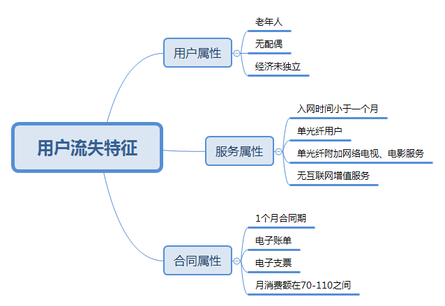
Through the above analysis, we can get the characteristics of the population with high loss rate. The population with these characteristics needs to manage it, increase user stickiness, and extend the life cycle value.
8, User churn forecast
1. Data preprocessing
The user ID column is useless. Delete it.
data.drop('user ID',inplace=True,axis=1)
Replace the value No phone service in the feature "whether the multi line service is enabled" with No,
Other features are treated the same way.
data['Whether multi line service has been opened'].replace('No phone service','No',inplace=True)
col=['Whether to open network security service','Whether to open online backup service','Whether the equipment protection business has been opened',
     'Whether the technical support service has been opened','Whether to open network TV','Open online movie or not']
for i in col:
    data[i].replace('No internet service','No',inplace=True
Observing the data type, we found that except for "customer access time", "monthly cost" and "total cost" are continuous features, the rest are basically discrete features. For discrete features, there is no size relationship between features. One hot coding is used, and there is size relationship between features, and numerical mapping is used.
clos=data[data.columns[data.dtypes==object]].copy()
for i in clos.columns:
    if clos[i].nunique()==2:
        clos[i]=pd.factorize(clos[i])[0]
    else:
        clos=pd.get_dummies(clos,columns=[i])
clos['aged']=data['aged']
clos['Monthly expenses']=data['Monthly expenses']
clos['Total cost']=data['Total cost']
clos['Access time of customers']=data['Access time of customers']
Divide features and labels.
X=clos.iloc[:,clos.columns!='Whether the user is lost']
y=clos.iloc[:,clos.columns=='Whether the user is lost'].values.ravel()
Sample balance processing: over sampling SMOTE algorithm is adopted, and its main principle is to insert data points in the neighborhood through interpolation.
print('Number of samples:{},1 occupy:{:.2%},0 occupy:{:.2%}'.format(X.shape[0],y.sum()/X.shape[0],(X.shape[0]-y.sum())/X.shape[0]))
smote=SMOTE(random_state=10)
over_X,over_y=smote.fit_sample(X,y)
print('Number of samples:{},1 occupy:{:.2%},0 occupy:{:.2%}'.format(over_X.shape[0],over_y.sum()/over_X.shape[0],(over_X.shape[0]-over_y.sum())/over_X.shape[0]))
#Operation result:
# Number of samples: 7043,1: 26.54%, 0: 73.46%
# Number of samples: 10348,1: 50.00%, 0: 50.00%
2. Model prediction
Partition training set test set.
Xtrain,Xtest,ytrain,ytest=train_test_split(over_X,over_y,test_size=0.3,random_state=10)
Decision tree, random forest, K-nearest neighbor and logistic regression are used. Observe the accuracy, accuracy, recall rate and f1 of the model.
model=[DecisionTreeClassifier(random_state=120)
      , RandomForestClassifier(random_state=120)
      ,KNeighborsClassifier()
      , LogisticRegression(max_iter=1000)]
for clf in model:
    clf.fit(Xtrain,ytrain)
    y_pre=clf.predict(Xtest)
    precision = precision_score(ytest, y_pre)
    accuracy = accuracy_score(ytest, y_pre)

    print(clf,'\n \n',classification_report(ytest,y_pre)
         ,'\n \n Precision Score:', precision
         ,'\n Accuracy Score::',accuracy
          ,'\n\n')
#Operation result:
DecisionTreeClassifier(ccp_alpha=0.0, class_weight=None, criterion='gini',
                       max_depth=None, max_features=None, max_leaf_nodes=None,
                       min_impurity_decrease=0.0, min_impurity_split=None,
                       min_samples_leaf=1, min_samples_split=2,
                       min_weight_fraction_leaf=0.0, presort='deprecated',
                       random_state=120, splitter='best')

               precision    recall  f1-score   support

           0       0.82      0.80      0.81      1581
           1       0.80      0.82      0.81      1524

    accuracy                           0.81      3105
   macro avg       0.81      0.81      0.81      3105
weighted avg       0.81      0.81      0.81      3105


 Precision Score: 0.7972027972027972
 Accuracy Score:: 0.8103059581320451


RandomForestClassifier(bootstrap=True, ccp_alpha=0.0, class_weight=None,
                       criterion='gini', max_depth=None, max_features='auto',
                       max_leaf_nodes=None, max_samples=None,
                       min_impurity_decrease=0.0, min_impurity_split=None,
                       min_samples_leaf=1, min_samples_split=2,
                       min_weight_fraction_leaf=0.0, n_estimators=100,
                       n_jobs=None, oob_score=False, random_state=120,
                       verbose=0, warm_start=False)

               precision    recall  f1-score   support

           0       0.85      0.86      0.85      1581
           1       0.85      0.84      0.85      1524

    accuracy                           0.85      3105
   macro avg       0.85      0.85      0.85      3105
weighted avg       0.85      0.85      0.85      3105


 Precision Score: 0.852589641434263
 Accuracy Score:: 0.851207729468599


KNeighborsClassifier(algorithm='auto', leaf_size=30, metric='minkowski',
                     metric_params=None, n_jobs=None, n_neighbors=5, p=2,
                     weights='uniform')

               precision    recall  f1-score   support

           0       0.82      0.70      0.75      1581
           1       0.73      0.84      0.78      1524

    accuracy                           0.77      3105
   macro avg       0.77      0.77      0.77      3105
weighted avg       0.77      0.77      0.77      3105


 Precision Score: 0.7269121813031162
 Accuracy Score:: 0.7671497584541063


LogisticRegression(C=1.0, class_weight=None, dual=False, fit_intercept=True,
                   intercept_scaling=1, l1_ratio=None, max_iter=1000,
                   multi_class='auto', n_jobs=None, penalty='l2',
                   random_state=None, solver='lbfgs', tol=0.0001, verbose=0,
                   warm_start=False)

               precision    recall  f1-score   support

           0       0.85      0.84      0.84      1581
           1       0.84      0.84      0.84      1524

    accuracy                           0.84      3105
   macro avg       0.84      0.84      0.84      3105
weighted avg       0.84      0.84      0.84      3105


 Precision Score: 0.8369210697977821
 Accuracy Score:: 0.8418679549114332
Draw the learning curve of the model and observe the fitting of the model.
figure,ax=plt.subplots(1,4,figsize=(30,4))
for i in range(4):
    train_sizes, train_scores, valid_scores=learning_curve(model[i],over_X,over_y, cv=5,random_state=10)
    train_std=train_scores.mean(axis=1)
    test_std=valid_scores.mean(axis=1)
    ax[i].plot(train_sizes,train_std,color='red',label='train_scores')
    ax[i].plot(train_sizes,test_std,color='blue',label='test_scores')
plt.legend()
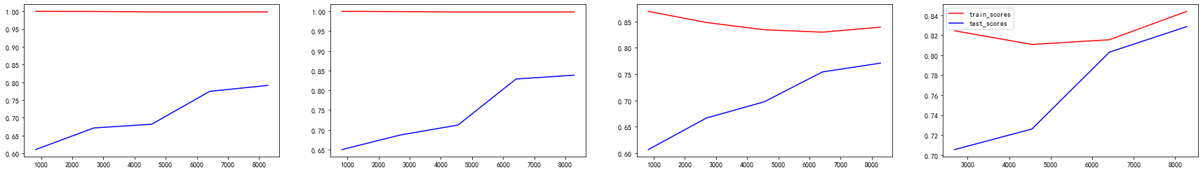
From the results, the accuracy, accuracy and f1 score of the prediction of random forest model are high, but there are serious over fitting. Next, we use grid search to adjust the parameters of random forest and reduce the over fitting.
param_grid  = {
                'n_estimators' : [500,1200],
#                'min_samples_split': [2,5,10,15],
#                'min_samples_leaf': [1,2,5,10],
                'max_depth': range(1,10,2),
#                 'max_features' : ('log2', 'sqrt'),
              }
rfc=RandomForestClassifier(random_state=120)
gridsearch = GridSearchCV(estimator =rfc, param_grid=param_grid,cv=5)
gridsearch.fit(Xtrain,ytrain)
print('best_params:',gridsearch.best_params_
      ,'\n \nbest_score: ',gridsearch.best_score_)
#Operation result:
best_params: {'max_depth': 9, 'n_estimators': 500}
best_score:  0.8408114378748538
rfc=RandomForestClassifier(random_state=120,max_depth=9, n_estimators= 500)
train_sizes, train_scores, valid_scores=learning_curve(rfc,over_X,over_y, cv=5,random_state=10)
train_std=train_scores.mean(axis=1)
test_std=valid_scores.mean(axis=1)
plt.plot(train_sizes,train_std,color='red',label='train_scores')
plt.plot(train_sizes,test_std,color='blue',label='test_scores')
plt.legend()
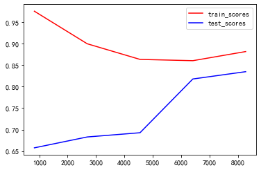
OK, after the parameter adjustment, the over fitting has been significantly reduced. Calculate the value of F1.
rfc=RandomForestClassifier(random_state=120,max_depth=9, n_estimators= 500)
rfc.fit(Xtrain,ytrain)
y_pre=rfc.predict(Xtest)
f1_score(ytest,y_pre)
#Operation result: 0.8451776649746194
3. Importance of features
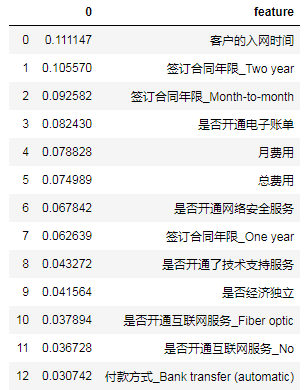
View the importance of features and sort them.
fea_import=pd.DataFrame(rfc.feature_importances_)
fea_import['feature']=list(Xtrain)
fea_import.sort_values(0,ascending=False,inplace=True)
fea_import.reset_index(drop=True,inplace=True)
fea_import
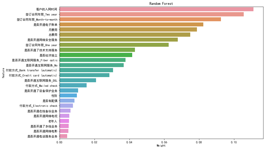
Visualize it.
figuer,ax=plt.subplots(figsize=(12,8))
g=sns.barplot(0,'feature',data=fea_import)
g.set_xlabel('Weight')
g.set_title('Random Forest')
9, Analysis suggestions
Based on the above analysis, suggestions are given from the perspective of business:
- According to the prediction model, a user list with high churn rate is constructed. A minimum feasible product function is launched through user research, and seed users are required to try it.
- Users: for the elderly users, no relatives and no partner users, develop exclusive personalized services, such as family packages, warm packages, etc., to improve the user experience.
- Service: for new registered users, push half a year's discount, such as giving consumption coupons, to tide over the peak of user loss. For optical fiber users and additional network TV and film users, the focus is to improve the network experience and value-added service experience, such as commitment to free network upgrade services for users. For online security, online backup, equipment protection, technical support and other value-added services, users should be focused on promotion and introduction, such as the first month / half year free experience.
- Contract aspect: for single month contract users, it is recommended to launch the half year contract payment discount activity to convert monthly users into half year users, improve the online time of users and increase the stickiness of users. For users who use electronic check, it is recommended to push coupons of other payment methods to guide users to change payment methods.