Learning today

Part I: pandas package

1, Introduction to pandas
pandas: a set of tools for analyzing structured data in python.
Based on numpy: providing high performance matrix operation
Graph library matplotlib: provide data visualization

2, pandas basic operation
1. Creation and basic operation of one-dimensional and two-dimensional arrays:

import numpy as np
import pandas as pd
s = pd.Series([1,2,3,4,np.NaN]) #One dimensional data Series in pandas
dates = pd.date_range('20200301',periods=6)
# Two dimensional array DataFrame, row index and column index in pandas

#Create DataFrame method 1:
data = pd.DataFrame(np.random.randn(6,4),index=dates,columns=list('abcd'))
data
Out[12]: 
                   a         b         c         d
2020-03-01  0.974217  1.415198  0.449173  0.309444
2020-03-02 -0.783394  1.642082  1.929648 -1.730744
2020-03-03 -1.412779  2.459838  0.793193  1.093348
2020-03-04 -2.860147 -1.633533  1.972606 -1.106984
2020-03-05  1.312970 -0.240283 -0.411076 -0.175680
2020-03-06 -0.277543 -0.525772  0.556319  0.938473

#Create DataFrame method 2:
d = {'A':1,'B':pd.Timestamp('20200301'),'C':range(4)}
df = pd.DataFrame(d,index = list('abcd'))
df
Out[16]: 
   A          B  C
a  1 2020-03-01  0
b  1 2020-03-01  1
c  1 2020-03-01  2
d  1 2020-03-01  3
------------------------
df.head(2)  #Output first 2 lines, default 5 lines
Out[25]: 
   A          B  C
a  1 2020-03-01  0
b  1 2020-03-01  1
df.tail(1)    #1 line after output, 5 lines by default
Out[26]: 
   A          B  C
d  1 2020-03-01  3

For a 2D array df:
df.index ---- return row index
df.columns ---- return column index
df.values ---- array of returned values
df.describe() -- return some data of the array

2. ranking:
1) Sort by index, axis=0 by column index, axis=1 by row index, and acsending is in ascending order. The default is True:

data.sort_index(axis=1,ascending=False)
Out[30]: 
                   d         c         b         a
2020-03-01  0.309444  0.449173  1.415198  0.974217
2020-03-02 -1.730744  1.929648  1.642082 -0.783394
2020-03-03  1.093348  0.793193  2.459838 -1.412779
2020-03-04 -1.106984  1.972606 -1.633533 -2.860147
2020-03-05 -0.175680 -0.411076 -0.240283  1.312970
2020-03-06  0.938473  0.556319 -0.525772 -0.277543

2) Sort by value:

data.sort_values(by='a')
Out[34]: 
                   a         b         c         d
2020-03-04 -2.860147 -1.633533  1.972606 -1.106984
2020-03-03 -1.412779  2.459838  0.793193  1.093348
2020-03-02 -0.783394  1.642082  1.929648 -1.730744
2020-03-06 -0.277543 -0.525772  0.556319  0.938473
2020-03-01  0.974217  1.415198  0.449173  0.309444
2020-03-05  1.312970 -0.240283 -0.411076 -0.175680

3. Selection: compared with the slower location index data[2:4], the index speed is faster through tag. loc() and number. iloc() (judgment is omitted):

data.loc[:,['b','c']]
Out[46]: 
                   b         c
2020-03-01  1.415198  0.449173
2020-03-02  1.642082  1.929648
2020-03-03  2.459838  0.793193
2020-03-04 -1.633533  1.972606
2020-03-05 -0.240283 -0.411076
2020-03-06 -0.525772  0.556319

data.iloc[1:3,:3]
Out[47]: 
                   a         b         c
2020-03-02 -0.783394  1.642082  1.929648
2020-03-03 -1.412779  2.459838  0.793193

4. Processing of DataFrame data:

For the processing of np.NaN (not a number), NaN does not participate in the calculation:
df1.dropna(how='any '). If there is NaN, the whole line will be discarded
 df1.fillna(value=5) × replace NaN with a value

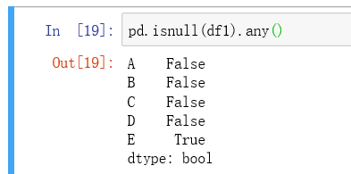
5. The difference between. any() and. all():
. any() -- treat a sequence as a whole and return True if one of the conditions is satisfied
. all() -- treat a sequence as a whole, and return True if each of them meets the conditions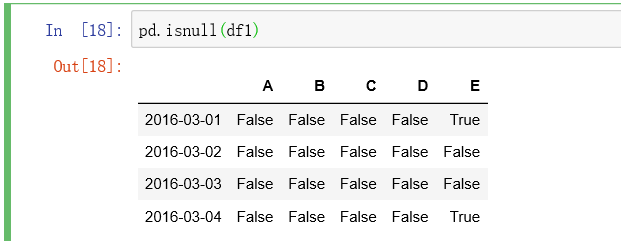


6. statistics:
df1.mean(axis=1) --- returns an array of average values per row (default axis=0, return average values per column)
df1.sum(axis=1) --- returns the array of the sum of values in each row (default axis=0, returns the sum of values in each column)
df.sub(s, axis = 'index') -- subtract s array from 2D array df by column
df.apply(func) --- incoming function. By default, the data in each column is transferred into the function (axis=0). The apply function will traverse the data in each row of DataFrame and return a Series data structure

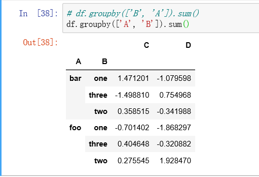
Group statistics:
df.groupby('A ') or df.groupby(['A','b ']) -- group with label A, or labels A and B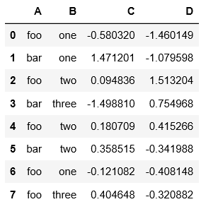


7. Data consolidation:
1) Vertical merge: pd.concat([xxx,xxx])
df1 = pd.concat([df.iloc[:3], df.iloc[3:7], df.iloc[7:]])
2) Merge with column label: pd.merge()
pd.merge(left, right, on = 'key') -- merge left and right according to 'key'
3) Add a row of data:
df.append(s,ignore_index=True)

8. Data perspective:
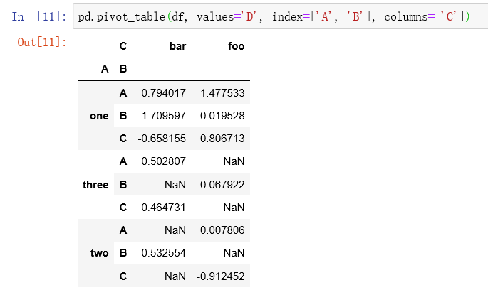
1)pivot table / axial rotation table:
PD. Pivot table (df, values = 'd', index = ['a ','b'], columns = ['c ') -- operate on df. The value is the value of column D, row index is the value of column A and B, and column index is the value of column C.


2)df[df.A = = 'one']. groupby('c '). mean() -- for the row with a column as one in df, group by the value of C column, and return the average value of D and E columns.

9. Time series:
rng = pd.date_range('20160301 ', periods=600, freq =' s') -- in date form, cycle is 600, unit is s second, default is' D ', unit is day.

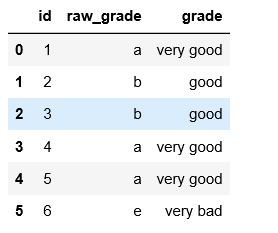
10.category:

df = pd.DataFrame({"id":[1,2,3,4,5,6], "raw_grade":['a', 'b', 'b', 'a', 'a', 'e']})
df["grade"] = df["raw_grade"].astype("category")
df["grade"].cat.categories
out: Index([u'a', u'b', u'e'], dtype='object')
df["grade"].cat.categories = ["very good", "good", "very bad"]