Basic concepts of greedy algorithm
"First of all, it should be emphasized that the premise of 01 knapsack problem is that each item has only two states: selected and not selected. Part of an item cannot be loaded into the knapsack. This is the meaning of 01 in 01 knapsack. If a part of an item can be loaded into the knapsack, a simpler idea than dynamic programming can be adopted: calculate each item through the value / weight of each item The value density of the item (my own term). Then take the item from high to low. This idea is a simple greedy algorithm idea. Because the item in the 01 knapsack problem can only be taken or not taken, when its capacity conflicts with the weight of the item, a simple greedy algorithm can not get the correct result“
In the previous chapter, the greedy algorithm was briefly mentioned when introducing the 01 knapsack problem. In the ordinary knapsack problem, a variety of items are loaded into a knapsack with limited capacity. Each item has two attributes of weight and value, and is allowed to be split. It is required to calculate the maximum value that the knapsack can hold. Think with greedy ideas, Obviously, we should give priority to loading items with greater value per unit weight. According to this idea, we can easily solve the knapsack problem
Greedy algorithm can be understood as selecting the local optimal solution in each part and obtaining the overall optimal solution. Of course, in many cases, the result obtained by greedy algorithm is not the real optimal solution, because the problem may be dynamic programming, which is a more valuable algorithm. However, The results obtained by dynamic programming are often close to the optimal solution. Therefore, greedy algorithm can be used as a cheating means for dynamic programming problems when the state transition equation cannot be found. With so many test points, there must be greedy algorithm that happens to be the optimal solution
Of course, without talking about these heresy, greedy algorithm is also of far-reaching significance. It is more an idea to solve problems. For example, Dijkstra algorithm, an important algorithm for single source shortest path problem, Prim algorithm and Kruskal algorithm for minimum spanning tree problem all adopt greedy idea. Today we try to understand greedy algorithm, It is also mainly carried out through the above three algorithms. It should be noted that due to the limitations of the author's energy and ability, my description of the above algorithm may be relatively abstract and there will not be too many vivid simulation processes. If the reader feels difficult to understand, I will attach the recommended Learning link address
Dijikstra algorithm to solve the single source shortest path problem
Description of single source shortest path problem:
In a graph, find the length of the shortest path from a point to all other points
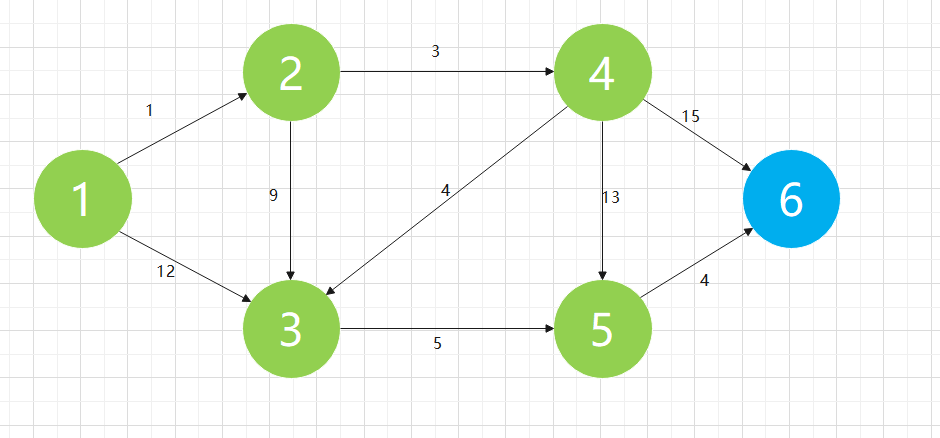
Here, we use the following legend to simulate the algorithm process. As shown in the figure below, a graph includes multiple edges, and each edge has different weights. The so-called shortest path is the minimum sum of the weights of the edges passing from one point to another. We need to find the shortest path length from node 1 to all other points
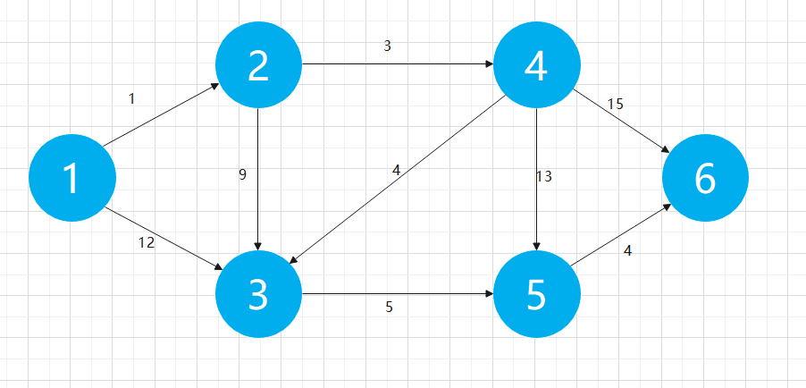
For this Graph, we can store it in the form of adjacency matrix. Here we set it as Graph [] [], where Graph[i][j] represents the edge weight from node i to node j. for two nodes that are not directly connected, the edge weight between them is considered infinite. The following table is our initial Graph [] [] adjacency matrix for this case
| 1 | 2 | 3 | 4 | 5 | 6 | |
| 1 | 0 | 1 | 2 | MAX_INT | MAX_INT | MAX_INT |
| 2 | MAX_INT | 0 | 9 | 3 | MAX_INT | MAX_INT |
| 3 | MAX_INT | MAX_INT | 0 | MAX_INT | 5 | MAX_INT |
| 4 | MAX_INT | MAX_INT | 4 | 0 | 13 | 15 |
| 5 | MAX_INT | MAX_INT | MAX_INT | MAX_INT | 0 | 4 |
| 6 | MAX_INT | MAX_INT | MAX_INT | MAX_INT | MAX_INT | 0 |
In addition, we need a one-dimensional array optimum [], where optimum[p] represents the shortest path length from node 1 to node p. in the initial state, only the nodes directly connected to node 1 have a current shortest path. With our calculation, the optimum [] array is gradually filled. When each node is marked as OK, the value of the optimum [] array will be determined, The following figure shows our initial optimization [] array in this case
| 1 | 2 | 3 | 4 | 5 | 6 |
| 0 | 1 | 12 | MAX_INT | MAX_INT | MAX_INT |
The reason why the greedy idea is applied to Dijikstra algorithm is that in each step of Dijikstra algorithm, if the optimal[x] in this step is the shortest path, then we think that the path from initial node 1 to node X has been determined. This idea of taking the local optimal solution is a greedy idea
Process simulation of Dijikstra algorithm
Let's simulate the process of Dijikstra algorithm:
Step 1:
For the initial state of the optimization array:
| 1 | 2 | 3 | 4 | 5 | 6 |
| 0 | 1 | 12 | MAX_INT | MAX_INT | MAX_INT |
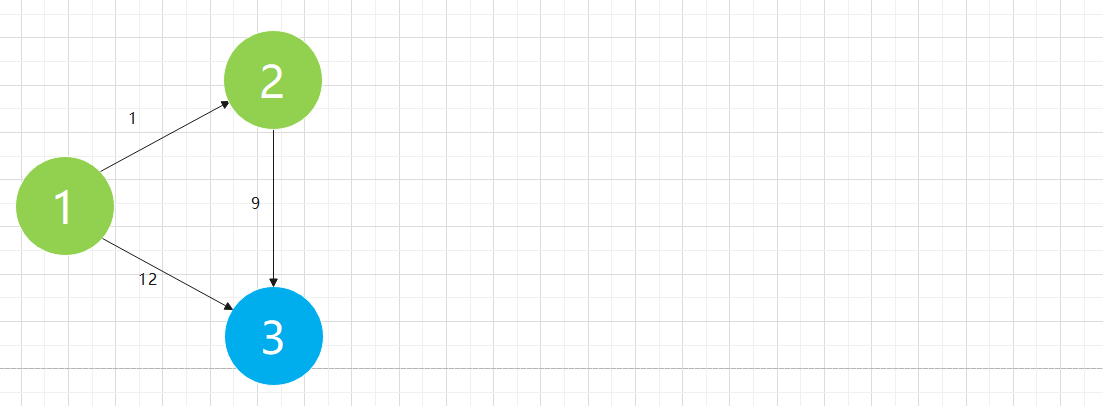
Except that the distance between node 1 and itself is 0, we find that the current shortest path is the path of 1 - > 2, and the distance is 1. Then we think that the shortest path of 1 - > 2 has been determined to be 1. We add node 2 to the determined graph
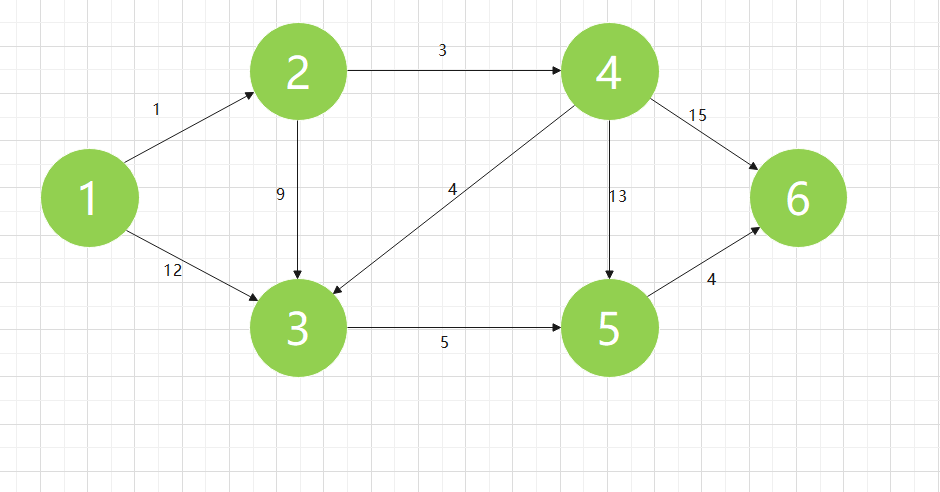
We can understand that only the following partial graphs are considered at present, in which the green node represents the set with the shortest path determined:
 Step 2:
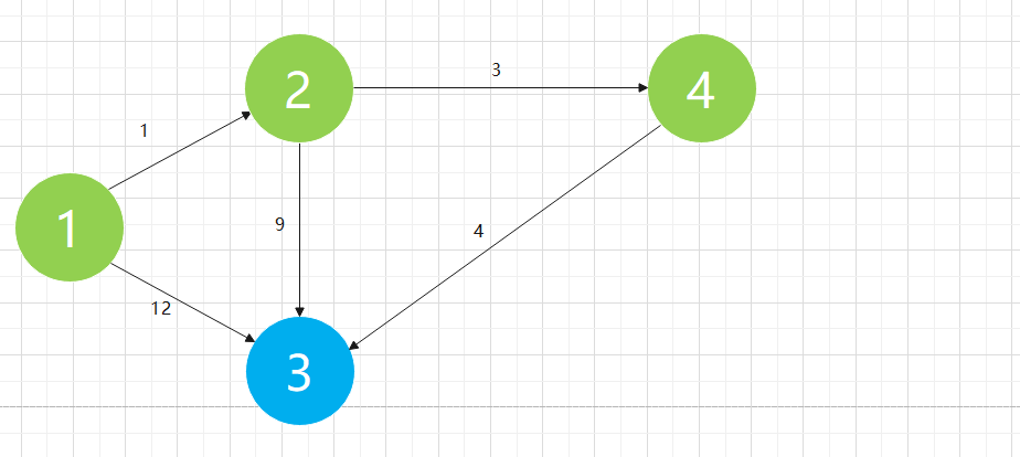
Now that node 2 has been determined, it is advisable to add the directly adjacent nodes of node 2 to the optimization [] array. If 1 - > 2 is the shortest, the adjacent nodes of 1 - > 2 may also have the shortest path. First, 2 - > 3, and graph [2] [3] + optimization [2] = 1 + 9 = 10 < optimization [3] = 12. Second, 2 - > 4, and graph [2] [4] + optimization [2] = 1 + 3 = 4 < optimization [4] = max_ Int, these two points obtain shorter paths through the newly added node 2, so we need to modify the relevant values of optimization []:
| 1 | 2 | 3 | 4 | 5 | 6 |
| 0 | 1 | 10 | 4 | MAX_INT | MAX_INT |
In addition to the determined nodes 1 and 2, we find that node 4 has the shortest path with optimization [4] = 4. We believe that the shortest path of node 4 has been determined
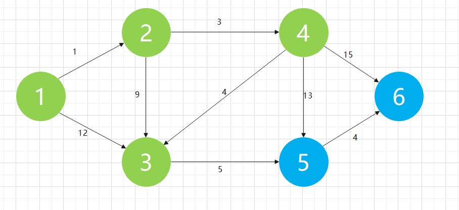
According to the above algorithm process, we continue to simulate and analyze in detail
Step 3:
| 1 | 2 | 3 | 4 | 5 | 6 |
| 0 | 1 | 8 | 4 | 17 | 19 |
Step 4:
| 1 | 2 | 3 | 4 | 5 | 6 |
| 0 | 1 | 8 | 4 | 13 | 19 |
Step 5:
| 1 | 2 | 3 | 4 | 5 | 6 |
| 0 | 1 | 8 | 4 | 13 | 17 |
So far, each node has been added to our determined set, that is, each element in the optimization [] array has been the value of the shortest path. This is the process of Dijikstra algorithm
Coding implementation of Dijikstra algorithm
The implementation of Dijikstra algorithm is as follows:
void Dijkstra(int u,bool* vis,int* optimum,int Graph[][]){
	for(int t=1;t<=n;t++){
		optimum[t]=Graph[u][t];
	}
	vis[u]=1;                        //The vis [] array marks the nodes that have been determined
	for(int t=1;t<n;t++)
	{
		int minn=Inf,temp;
		for(int i=1;i<=n;i++)       //Find out which node is the shortest path to at this step
		{
			if(!vis[i]&&optimum[i]<minn)//The current node has not been determined, and the shortest path to the current node is the smallest
			{
				minn=optimum[i];
				temp=i;
			}
		}
		vis[temp]=1;
		for(int i=1;i<=n;i++)
		{
			if(Graph[temp][i]+optimum[temp]<optimum[i])  //The addition of new nodes results in a shorter path length
			{
				optimum[i]=Graph[temp][i]+optimum[temp];
			}
		}
	}

}
Minimum spanning tree problem
Minimum spanning tree problem description
In all spanning trees of a connected network, the cost of all edges and the smallest spanning tree are called the minimum spanning tree. Our goal is to find a minimum spanning tree in a connected graph.
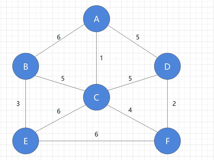
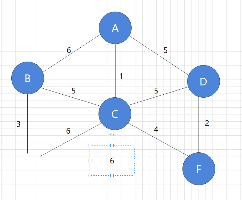
For example, for the following figure:
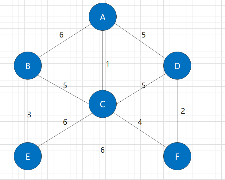
There is a minimum spanning tree:
Facing this problem, there are two classical algorithms: Prim algorithm and Kruskal algorithm. Next, we will discuss the implementation of the two algorithms and their relationship.
Kruskal algorithm
Kruskal algorithm process simulation:
Kruskal algorithm can be understood as edging method. In the initial state, we consider that all nodes exist in isolation, and then add edges from short to long to the graph until the graph becomes a connected graph. This is also a typical greedy idea: I hope the total length of the path is the shortest, so at each step, I hope to get the shortest path as possible.
It should be noted that in addition to ensuring that the newly added edge is the shortest, it should also ensure that the newly added edge can connect two connected components. If the addition of this edge can not reduce the number of connected components, it is meaningless.
Let's simulate this process:
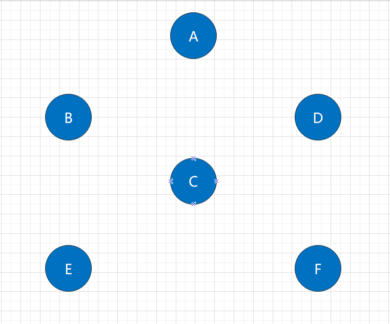
Initial state:
At this point, the points in the graph exist in isolation. Next, we need to add edges in the figure:
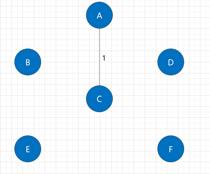
 Step 1:
Obviously, in the original graph, the shortest edge is the edge of A-C, with A length of 1. At the same time, its addition also connects the two connected components of A and C.
After adding this edge, it is obvious that this graph is still not a connected graph. So we need to continue the algorithm.
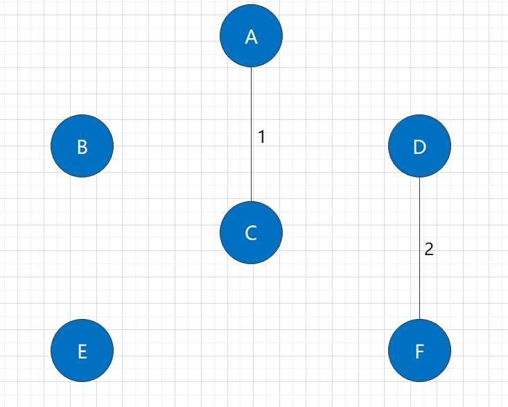
Step 2:
Among the unused edges in the figure, the shortest is the D-F edge, with a length of 2. It obviously also connects two connected components.
After adding this edge, it is still not a connected graph, so we need to continue the algorithm.
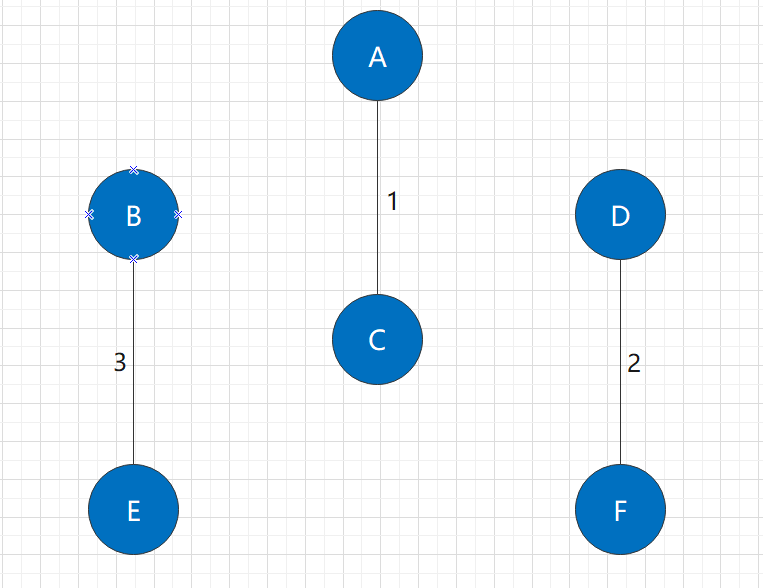
Step 3:
Among the unused edges in the figure, the shortest is the B-E edge with a length of 3. It obviously also connects two connected components.
After adding this edge, it is still not a connected graph, so we need to continue the algorithm.
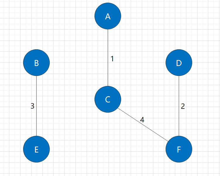
Step 4:
Among the unused edges in the figure, the shortest is the C-F edge, with a length of 4. It obviously also connects two connected components.
After adding this edge, it is still not a connected graph, so we need to continue the algorithm.
Step 5:
Among the unused edges in the graph, the shortest ones are B-C edge and C-D edge, both of which are 5 in length. At this time, we need to select the edge that can reduce the number of connected components.
If I choose to add C-D edges:
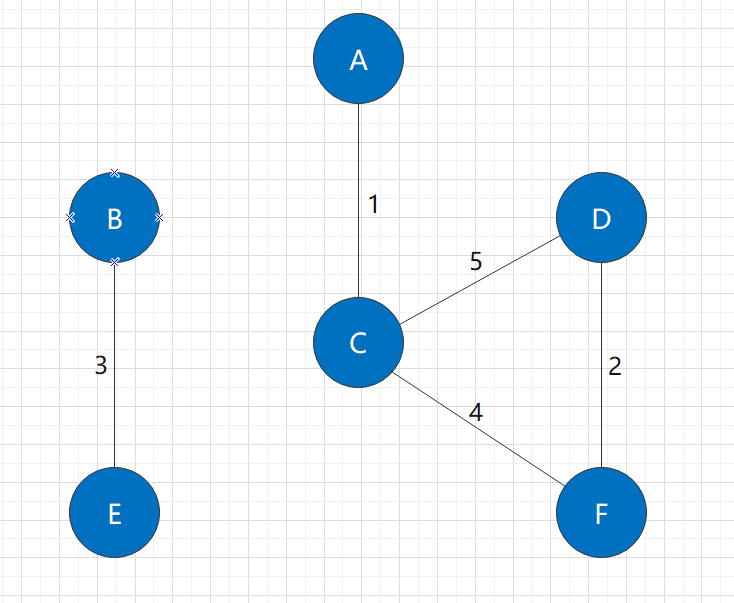 Before and after adding edges, there are two connected components, so this edge is meaningless, but increases the overhead of the path. In addition, there is a loop in the figure, and it is no longer a tree.
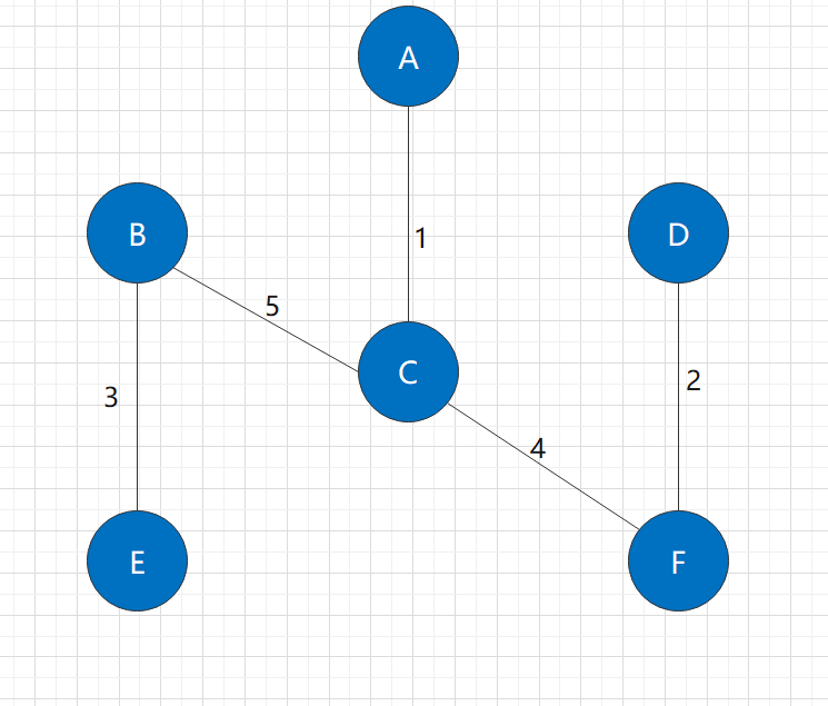
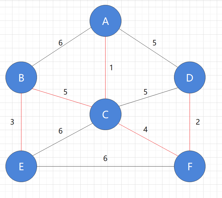
The selection of B-C edge can meet our requirements:
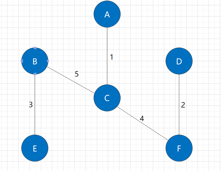
At this point, the whole graph is connected and the algorithm ends. In this process, the graph we generate is the minimum spanning tree that meets the requirements.
Coding implementation of Kruskal algorithm:
Kruskal algorithm is not the kind of algorithm that can be easily coded after understanding the principle. In coding, we face many difficulties
1. How to store a graph?
The simplest way is to store it through an adjacency matrix. However, for this topic, we need to select the shortest edge, and then the sub shortest edge... If the adjacency matrix is used, we need to traverse the two-dimensional array every time we select the edge, This is an unacceptable time complexity. Therefore, we adopt an edge centered storage method: store all edges through a one-dimensional array. An edge can be composed of two endpoints and its length, so the implementation of this data structure is as follows:
struct edge{		//Storing edges in a graph
	int pointA;
	int pointB;
	int value;
};

edge e[N];
In this way, we only need to sort the e [] array of saved edges according to the value value, and we can easily take out the edges in the graph by length
2. How to describe the connectivity of graphs? How to determine whether the newly added edges reduce the number of connected components of the graph?
This paper introduces a very important sub algorithm to solve the connectivity problem of graphs: union search set algorithm. Union search set is an important algorithm specially used to maintain the connectivity of graphs or judge whether there are rings in graphs. As the name suggests, union search set is the merging and query operation of sets. The content of union search set can be regarded as an independent subject, Here we are on the topic. It is enough to maintain the set of nodes
To use the joint query set, we should regard each connected component as a tree and judge whether the two nodes are in the same connected component. In essence, it is to judge whether the root nodes of the tree where the two nodes are located are the same. The code to realize this process is given below:
First, the parent node of each node is stored through the par [] array. If it is the root node, the parent node is itself
int par[N];
int high[N];
For this topic, in the initial state, each node is a tree and is the parent node. With the edge added to the graph, the tree needs to be merged. The following code implements this process
void init(int n,int* par,int* high){	//Initialize the union query set of n nodes
	for(int i=0;i<n;i++){
		par[i]=i;						//In the initial state, the parents of each node are themselves
		high[i]=0;						//In the initial state, the height of each node is 0
	}
}
int findPar(int p,int* par){						//Find the root of a node
	return par[p]==p?p:findPar(par[p],par);//If the parent of the current node is itself, return its own number; otherwise, find its parent node
}
void merge(int x,int y,int* par,int* high){				//Merge two sets
	x=findPar(x,par);						//Find the root node of the two nodes
	y=findPar(y,par);
	if(x==y) return;					//The two nodes have the same root. Return directly
	if(high[x]<high[y]) par[x]=y;		//If the Y node is higher, set the father of x to y
	else if(high[y]<high[x]){
		par[y]=x;
	}else{
		high[x]++;						//If the two heights are different, increase the height of x and set y's parents to x
		par[y]=x;
	}
}
The overall code of this topic is given below:
#include<iostream>
#include<algorithm>
using namespace std;
#define N 100
#define INF MAX_INT
struct edge{		//Storing edges in a graph
	int pointA;
	int pointB;
	int value;
};
void init(int n,int* par,int* high){	//Initialize the union query set of n nodes
	for(int i=0;i<n;i++){
		par[i]=i;						//In the initial state, the parents of each node are themselves
		high[i]=0;						//In the initial state, the height of each node is 0
	}
}
void initEdge(int n,int m,edge* e){				//The initialization diagram, where the static diagram is injected directly, is the example shown above
	e[0].pointA=1;
	e[0].pointB=2;
	e[0].value=6;

	e[1].pointA=1;
	e[1].pointB=3;
	e[1].value=1;

	e[2].pointA=1;
	e[2].pointB=4;
	e[2].value=5;

	e[3].pointA=2;
	e[3].pointB=3;
	e[3].value=5;

	e[4].pointA=3;
	e[4].pointB=4;
	e[4].value=5;

	e[5].pointA=2;
	e[5].pointB=5;
	e[5].value=3;

	e[6].pointA=3;
	e[6].pointB=5;
	e[6].value=6;

	e[7].pointA=5;
	e[7].pointB=6;
	e[7].value=6;

	e[8].pointA=3;
	e[8].pointB=6;
	e[8].value=4;

	e[9].pointA=4;
	e[9].pointB=6;
	e[9].value=2;
}
int findPar(int p,int* par){						//Find the root of a node
	return par[p]==p?p:findPar(par[p],par);//If the parent of the current node is itself, return its own number; otherwise, find its parent node
}
void merge(int x,int y,int* par,int* high){				//Merge two sets
	x=findPar(x,par);						//Find the root node of the two nodes
	y=findPar(y,par);
	if(x==y) return;					//The two nodes have the same root. Return directly
	if(high[x]<high[y]) par[x]=y;		//If the Y node is higher, set the father of x to y
	else if(high[y]<high[x]){
		par[y]=x;
	}else{
		high[x]++;						//If the two heights are different, increase the height of x and set y's parents to x
		par[y]=x;
	}
}
bool same(int x,int y){
	return findPar[x]==findPar[y];
}
bool cmp(edge a,edge b){
	return a.value<b.value;
}
void kruskal(int n,int m,int* par,int* high,edge* e){//n points, m edges, kruskal algorithm
	int sumValue=0;		//Total weight
	int numEdge=0;		//The total number of edges. Obviously, in the minimum spanning tree, the number of edges is - 1
	sort(e,e+m,cmp);//The m edges in the graph are arranged in ascending order
	init(n,par,high);					//Initialize and query set
	for(int i=0;i<m;i++){				//Turn the edge from short to long
		int pointA=e[i].pointA;
		int pointB=e[i].pointB;
		if(findPar[pointA-1]!=findPar[pointB-1]){	//The starting point of the following table is 0 and the node starting point of the graph is 1. When the root nodes of two points are different, the edges are added to the result set and the two sets are merged
			cout<<pointA<<" "<<pointB<<" "<<e[i].value<<endl;
			sumValue+=e[i].value;
			numEdge++;
			merge(pointA-1,pointB-1,par,high);			//Merge two sets
		}
		if(numEdge>=n-1){		//When the added edge reaches n-1, it must have met the requirements and exit the cycle directly
			break;
		}
	}
	cout<<"The total value of the minimum spanning tree is:"<<sumValue<<endl;
	return;
}
int main(){
	edge e[N];
	int n=6;
	int m=10;
	int par[N];
	int high[N];
	initEdge(6,10,e);			//Initialization diagram
	kruskal(n,m,par,high,e);
	return 0;
}
Finally, the attributes of the edges reserved in the minimum spanning tree are output
Prim algorithm
Prim algorithm process simulation
Prim algorithm can be understood as adding points method. In the initial state, we think that there is only one node in the graph, and then add nodes connected to the shortest edge according to the shortest edge in the current graph until all points in the original graph are connected to each other to obtain our minimum spanning tree
Corresponding to Kruskal algorithm, when selecting the shortest edge, it is necessary to ensure that the node connected by the shortest edge has not been connected, otherwise this edge will be meaningless
Let's simulate this process:
Still use this figure as an example:
Initial state:
We start the algorithm with point A as the initial node. Of course, the minimum spanning tree can be obtained using any node
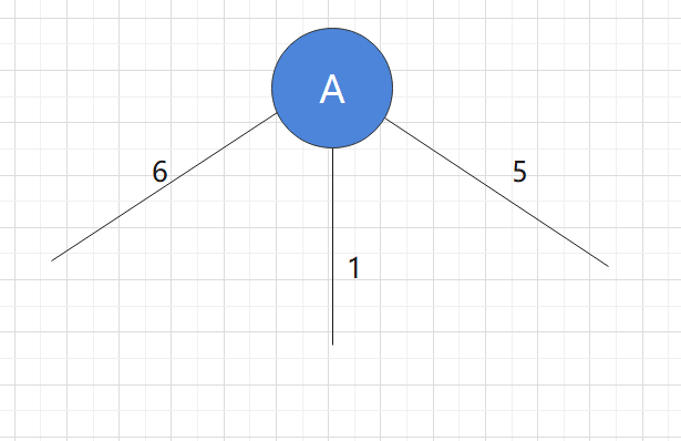
Step 1:
Observing the current graph, we find that the shortest edge is the one with the weight of 1, and the nodes connected by this edge must not have been added to the current graph. Therefore, we add the nodes connected by the edge with the length of 1 to the graph
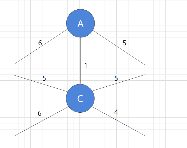
Step 2:
At this time, we observe all the edges in the graph and find that the shortest one is the one with length of 4. And the connected nodes have not been added to the graph, so we add new nodes to the graph
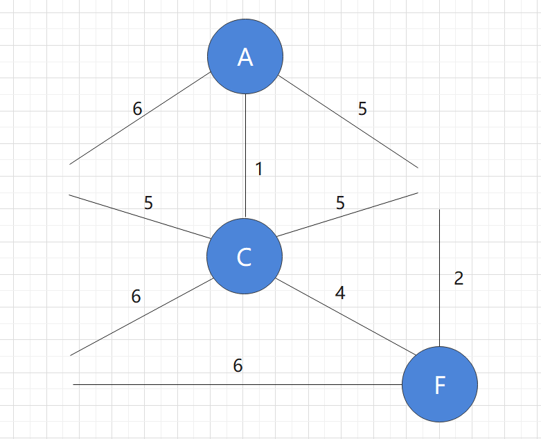
Step 3:
Similarly, add the points connected by edges with length 2 to the graph
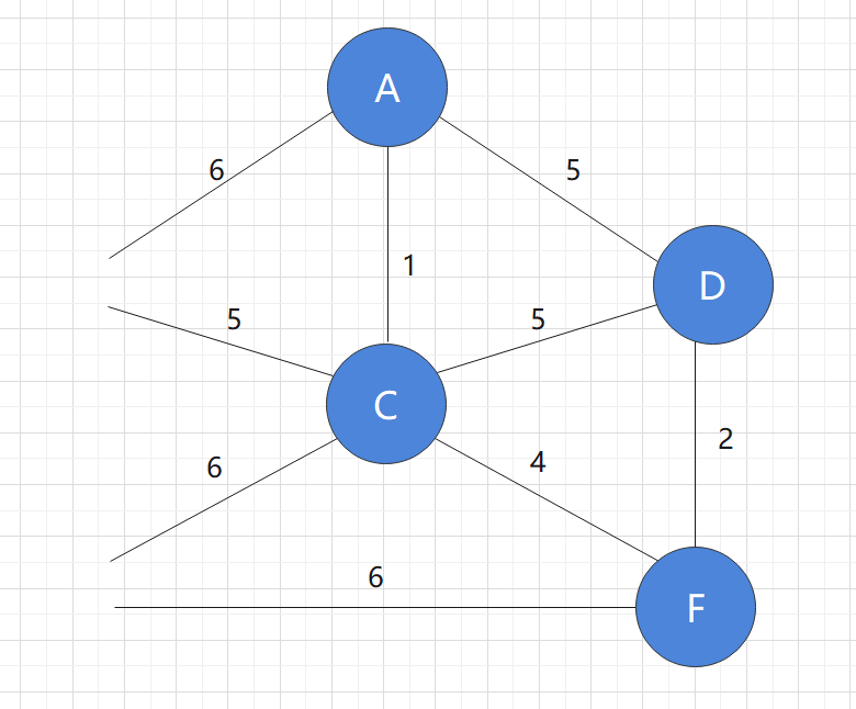
Step 4:
Step 5:
At this point, all nodes have been added to the graph. Mark the used edges and find that this is a minimum spanning tree
In addition, except for the red edges in the figure, none of the other edges are real. Only when adding new nodes, we need to consider these edges and draw them for easy observation
Coding implementation of Prim algorithm
The only thing to note is that according to the requirements of the topic, we use the nesting of point and edge structures in the storage graph this time. In fact, the complexity of this clock writing method is not different from that of adjacency matrix. When facing the topic of graph theory, the storage structure of graph is a point that needs to be cautious, and a good data structure can reduce the time complexity as much as possible
Compared with Kruskal algorithm, Prim algorithm does not have too many implementation difficulties, which will not be repeated here. The author's implementation code is directly displayed
The author did not make careful optimization. It can be seen that the time complexity of the algorithm can reach O(n^3) when searching the shortest node violently. The author is welcome to put forward the optimization scheme
#include<iostream>
#include<algorithm>
#include<vector>
using namespace std;
#define N 100
struct edge{
	int pointA;
	int pointB;
	int value;
};
struct point{		//Node structure, which can store the edges connected by this node
	edge e[N];
	int eNum;
};

bool cmp(edge a,edge b){
	return a.value<b.value;
}
void initPoints(point* p){	//Initialize the drawing and input the original drawing
	p[1].eNum=3;
	p[1].e[0].pointA=1;
	p[1].e[0].pointB=3;
	p[1].e[0].value=1;

	p[1].e[1].pointA=1;
	p[1].e[1].pointB=2;
	p[1].e[1].value=6;

	p[1].e[2].pointA=1;
	p[1].e[2].pointB=4;
	p[1].e[2].value=5;

	p[2].e[0].pointA=2;
	p[2].e[0].pointB=3;
	p[2].e[0].value=5;

	p[2].eNum=3;
	p[2].e[1].pointA=2;
	p[2].e[1].pointB=5;
	p[2].e[1].value=3;

	p[2].e[2].pointA=2;
	p[2].e[2].pointB=1;
	p[2].e[2].value=6;

	p[4].eNum=3;
	p[4].e[0].pointA=4;
	p[4].e[0].pointB=1;
	p[4].e[0].value=5;

	p[4].e[1].pointA=4;
	p[4].e[1].pointB=3;
	p[4].e[1].value=5;

	p[4].e[2].pointA=4;
	p[4].e[2].pointB=6;
	p[4].e[2].value=2;

	p[3].eNum=5;
	p[3].e[0].pointA=3;
	p[3].e[0].pointB=1;
	p[3].e[0].value=1;

	p[3].e[1].pointA=3;
	p[3].e[1].pointB=2;
	p[3].e[1].value=5;

	p[3].e[2].pointA=3;
	p[3].e[2].pointB=4;
	p[3].e[2].value=4;

	p[3].e[3].pointA=3;
	p[3].e[3].pointB=5;
	p[3].e[3].value=6;

	p[3].e[4].pointA=3;
	p[3].e[4].pointB=6;
	p[3].e[4].value=4;

	p[5].eNum=3;
	p[5].e[0].pointA=5;
	p[5].e[0].pointB=2;
	p[5].e[0].value=3;

	p[5].e[1].pointA=5;
	p[5].e[1].pointB=3;
	p[5].e[1].value=6;

	p[5].e[2].pointA=5;
	p[5].e[2].pointB=6;
	p[5].e[2].value=6;

	p[6].eNum=3;
	p[6].e[0].pointA=6;
	p[6].e[0].pointB=4;
	p[6].e[0].value=2;

	p[6].e[1].pointA=6;
	p[6].e[1].pointB=3;
	p[6].e[1].value=4;

	p[6].e[2].pointA=6;
	p[6].e[2].pointB=5;
	p[6].e[2].value=6;

	for(int i=1;i<=6;i++){
		sort(p[i].e,p[i].e+p[i].eNum-1,cmp);//Sort edges from short to long
	}
}
void prim(point* p,bool* visited,int visitedSum,vector<point>visitedPoints){
	while(visitedSum<6){
	edge minEdge;
	minEdge.value=0x4f;
	for(int i=0;i<visitedPoints.size();i++){
		 for(int j=0;j<visitedPoints[i].eNum;j++){			//Traverse to find the shortest edge currently
		 	if(visitedPoints[i].e[j].value<minEdge.value&&visited[visitedPoints[i].e[j].pointB]==false){
		 		minEdge=visitedPoints[i].e[j];
			 }
		 }
	}
	cout<<minEdge.pointA<<"---"<<minEdge.pointB<<" "<<minEdge.value<<endl;
	visited[minEdge.pointB]=true;
	visitedPoints.push_back(p[minEdge.pointB]);
	visitedSum++;
	}
}
int main(){
	point p[N];
	initPoints(p);				//Initialization diagram
	bool visited[6];
	vector<point>visitedPoints;	//Stores the points that have been traversed
	int visitedSum=1;			//In the initial state, only the first point has been traversed
	visited[1]=true;
	visitedPoints.push_back(p[1]);
	prim(p,visited,visitedSum,visitedPoints);
	return 0;
}
summary
We call a complete graph whose number of edges is far less than that of the same node as a sparse graph. A graph whose number of edges is close to that of a complete graph as a dense graph. Because Kruskal algorithm obtains the minimum spanning tree by adding edges, it will inevitably reduce the efficiency when there are too many edges, so Kruskal algorithm is more suitable for sparse graphs to find the minimum spanning tree. In comparison, Prim algorithm looks for nodes every time, Therefore, even when the graph is very dense, this idea can ignore many unnecessary nodes. Therefore, Prim algorithm is more suitable for finding the minimum spanning tree of dense graph. This is the main difference between the two in application