Advanced Neural Network

Experimental environment

keras 2.1.5
tensor 1.4.0

Experimental tools

Jupyter Notebook

Experiment 1: MNIST generates antagonistic networks

thinking

Work process: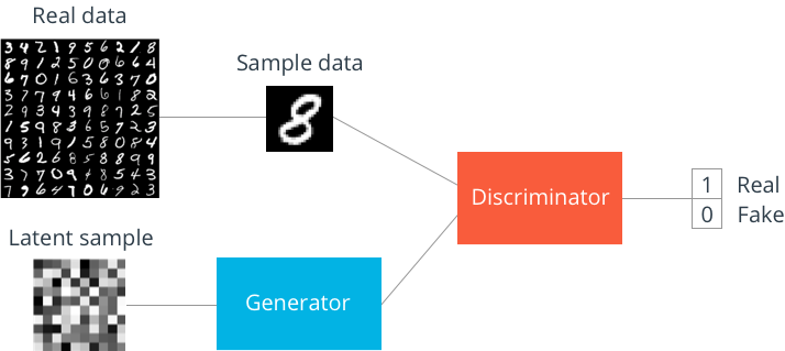

Experimental process

1. Load Dependencies:

%matplotlib inline

import numpy as np
import matplotlib.pyplot as plt

import keras
from keras.layers import Dense, Activation, Dropout, Flatten, Reshape, LeakyReLU 
from keras.layers import Conv2D, Conv2DTranspose, UpSampling2D, BatchNormalization
from keras.layers import Cropping2D
from keras.datasets import mnist
from keras.models import Sequential
from keras.optimizers import RMSprop

from sklearn.utils import shuffle

2. Loading and preparing datasets:

(x_train, y_train), (x_test, y_test) = mnist.load_data()
x_train = x_train.astype("float32")/255.

Although the images are grayscale, we will increase the channel dimension by 1 because the convolution layer requires them.

x_train = x_train.reshape((x_train.shape[0],x_train.shape[1],x_train.shape[2],1))
x_test = x_test.reshape((x_test.shape[0],x_test.shape[1],x_test.shape[2],1))

y_train = y_train.reshape((y_train.shape[0],-1))
y_test = y_test.reshape((y_test.shape[0],-1))

train_data_shape = x_train.shape
test_data_shape = x_test.shape

train_label_shape = y_train.shape
test_label_shape = y_test.shape
#Take a look at the output:
print("train data shape:",train_data_shape)
print("train label shape:",train_label_shape)
print("test data shape:",test_data_shape)
print("test label shape:",test_label_shape)
'''
train data shape: (60000, 28, 28, 1)
train label shape: (60000, 1)
test data shape: (10000, 28, 28, 1)
test label shape: (10000, 1)
'''

3. Establish a network model:
Discriminator:
We set up a discriminator network to receive [1,28,28] image vectors and determine whether they are true or false by using multiple convolution layers, dense layers, large loss, and two element Softmax output layer encoding: [0,1]=false and [1,0]=true.

D = Sequential()

dropout = 0.4

input_shape = train_data_shape[1:]

D.add(Conv2D(16, 3, strides=2, input_shape=input_shape,padding='same'))
D.add(LeakyReLU(alpha=0.2))

D.add(Dropout(dropout))

D.add(Conv2D(32, 3, strides=2, padding='same'))
D.add(LeakyReLU(alpha=0.2))

D.add(Dropout(dropout))

D.add(Conv2D(64, 3, strides=2, padding='same'))
D.add(LeakyReLU(alpha=0.2))

D.add(Dropout(dropout))

D.add(Flatten())

D.add(Dense(1))

D.add(Activation('sigmoid'))

D.summary()

optimizer1 = RMSprop(lr=0.0008, clipvalue=1.0, decay=6e-8)
D.compile(loss='binary_crossentropy', optimizer=optimizer1,metrics=['accuracy'])
'''
_________________________________________________________________
Layer (type)                 Output Shape              Param #   
=================================================================
conv2d_1 (Conv2D)            (None, 14, 14, 16)        160       
_________________________________________________________________
leaky_re_lu_1 (LeakyReLU)    (None, 14, 14, 16)        0         
_________________________________________________________________
dropout_1 (Dropout)          (None, 14, 14, 16)        0         
_________________________________________________________________
conv2d_2 (Conv2D)            (None, 7, 7, 32)          4640      
_________________________________________________________________
leaky_re_lu_2 (LeakyReLU)    (None, 7, 7, 32)          0         
_________________________________________________________________
dropout_2 (Dropout)          (None, 7, 7, 32)          0         
_________________________________________________________________
conv2d_3 (Conv2D)            (None, 4, 4, 64)          18496     
_________________________________________________________________
leaky_re_lu_3 (LeakyReLU)    (None, 4, 4, 64)          0         
_________________________________________________________________
dropout_3 (Dropout)          (None, 4, 4, 64)          0         
_________________________________________________________________
flatten_1 (Flatten)          (None, 1024)              0         
_________________________________________________________________
dense_1 (Dense)              (None, 1)                 1025      
_________________________________________________________________
activation_1 (Activation)    (None, 1)                 0         
=================================================================
Total params: 24,321
Trainable params: 24,321
Non-trainable params: 0
_________________________________________________________________
'''

Gernerator:
Using the function API, we built a relatively simple generation model in Keras, took 100 random inputs, and finally mapped them to a [1, 28, 28] pixel to match the shape of the MNIST data.First, a dense set of 14*14 values is generated, then several filters of different sizes and number of channels are run, and the use of binary cross-entropy and adam optimizer are trained.We use Sigmiod on the output layer to help saturate the pixels to a 0 or 1 state instead of a gray scale between 0 or 1, and batch normalization to help speed up training and ensure a wide range of activations are used in each layer.

G = Sequential()

dropout = 0.4

G.add(Dense(4*4*128, input_dim=100))
G.add(BatchNormalization(momentum=0.9))
G.add(Activation('relu'))

G.add(Reshape((4, 4, 128)))

G.add(UpSampling2D())
G.add(Conv2DTranspose(64, 3, padding='same'))
G.add(BatchNormalization(momentum=0.9))
G.add(Activation('relu'))

G.add(UpSampling2D())
G.add(Conv2DTranspose(32, 3, padding='same'))
G.add(BatchNormalization())
G.add(Activation('relu'))

G.add(UpSampling2D())

G.add(Cropping2D(cropping=((2, 2), (2, 2))))
      
G.add(Conv2DTranspose(16, 3, padding='same'))
G.add(BatchNormalization(momentum=0.9))
G.add(Activation('relu'))

G.add(Conv2DTranspose(8, 3, padding='same'))
G.add(BatchNormalization(momentum=0.9))
G.add(Activation('relu'))

G.add(Conv2DTranspose(1, 3, padding='same'))
G.add(Activation('sigmoid'))

G.summary()
'''
_________________________________________________________________
Layer (type)                 Output Shape              Param #   
=================================================================
dense_2 (Dense)              (None, 2048)              206848    
_________________________________________________________________
batch_normalization_1 (Batch (None, 2048)              8192      
_________________________________________________________________
activation_2 (Activation)    (None, 2048)              0         
_________________________________________________________________
reshape_1 (Reshape)          (None, 4, 4, 128)         0         
_________________________________________________________________
up_sampling2d_1 (UpSampling2 (None, 8, 8, 128)         0         
_________________________________________________________________
conv2d_transpose_1 (Conv2DTr (None, 8, 8, 64)          73792     
_________________________________________________________________
batch_normalization_2 (Batch (None, 8, 8, 64)          256       
_________________________________________________________________
activation_3 (Activation)    (None, 8, 8, 64)          0         
_________________________________________________________________
up_sampling2d_2 (UpSampling2 (None, 16, 16, 64)        0         
_________________________________________________________________
conv2d_transpose_2 (Conv2DTr (None, 16, 16, 32)        18464     
_________________________________________________________________
batch_normalization_3 (Batch (None, 16, 16, 32)        128       
_________________________________________________________________
activation_4 (Activation)    (None, 16, 16, 32)        0         
_________________________________________________________________
up_sampling2d_3 (UpSampling2 (None, 32, 32, 32)        0         
_________________________________________________________________
cropping2d_1 (Cropping2D)    (None, 28, 28, 32)        0         
_________________________________________________________________
conv2d_transpose_3 (Conv2DTr (None, 28, 28, 16)        4624      
_________________________________________________________________
batch_normalization_4 (Batch (None, 28, 28, 16)        64        
_________________________________________________________________
activation_5 (Activation)    (None, 28, 28, 16)        0         
_________________________________________________________________
conv2d_transpose_4 (Conv2DTr (None, 28, 28, 8)         1160      
_________________________________________________________________
batch_normalization_5 (Batch (None, 28, 28, 8)         32        
_________________________________________________________________
activation_6 (Activation)    (None, 28, 28, 8)         0         
_________________________________________________________________
conv2d_transpose_5 (Conv2DTr (None, 28, 28, 1)         73        
_________________________________________________________________
activation_7 (Activation)    (None, 28, 28, 1)         0         
=================================================================
Total params: 313,633
Trainable params: 309,297
Non-trainable params: 4,336
_________________________________________________________________
'''

Generate regression models:
Use the functional API to combine the generation model with the resistance model.

D.trainable = False  

gan = Sequential()
gan.add(G)
gan.add(D)
gan.summary()

optimizer2 = RMSprop(lr=0.0004, clipvalue=1.0, decay=3e-8)
gan.compile(loss='binary_crossentropy', optimizer=optimizer2, metrics=['accuracy'])
'''
_________________________________________________________________
Layer (type)                 Output Shape              Param #   
=================================================================
sequential_2 (Sequential)    (None, 28, 28, 1)         313633    
_________________________________________________________________
sequential_1 (Sequential)    (None, 1)                 24321     
=================================================================
Total params: 337,954
Trainable params: 309,297
Non-trainable params: 28,657
_________________________________________________________________
'''

4. Training:
Define a function to draw and save the output of the generator:

def plot_images(save2file=False, fake=True, samples=16, noise=None, step=0):
    filename = 'mnist.png'
    if fake:
        if noise is None:
            noise = np.random.uniform(-1.0, 1.0, size=[samples, 100])
        else:
            filename = "mnist_%d.png" % step
        images = G.predict(noise)
    else:
        i = np.random.randint(0, self.x_train.shape[0], samples)
        images = x_train[i, :, :, :]

    plt.figure(figsize=(10,10))
    for i in range(images.shape[0]):
        plt.subplot(4, 4, i+1)
        image = images[i, :, :, :]
        image = np.reshape(image, [train_data_shape[1], train_data_shape[2]])
        plt.imshow(image, cmap='gray')
        plt.axis('off')
    plt.tight_layout()
    if save2file:
        plt.savefig(filename)
        plt.close('all')
    else:
        plt.show()

Set superparameters:

save_interval = 20   #save a plot that includes the output of the generator every number of steps 
train_steps=2000      # end number of steps
start_step = 0        # start number of steps
batch_size=256       # batch size

Discriminant models are pre-trained, several random images are generated using untrained generation models, connected to the same number of real digital images, tagged appropriately, and fitted until we reach a relatively stable loss value, which exceeds 20,000 examples.

num_pretrain = 5000
images_train = x_train[np.random.randint(0,x_train.shape[0], size=num_pretrain), :, :, :]  #selecting random num_pretrain images from training data
noise = np.random.uniform(0, 1.0, size=[num_pretrain, 100])   #generating random num_pretrain noise vectors
images_fake = G.predict(noise)   #generating fake images from the generator
x = np.concatenate((images_train, images_fake))  #stacking both real and fake images
#generating labels in which real=1, fake =0
y = np.ones([2*num_pretrain, 1])
y[num_pretrain:, :] = 0

x,y = shuffle(x,y)  #shuffling the data and labels

d_loss = D.fit(x, y, batch_size=batch_size, epochs=1, validation_split=0.15) #the pretraining step
'''
Train on 8500 samples, validate on 1500 samples
Epoch 1/1
8500/8500 [==============================] - 3s 335us/step - loss: 0.1738 - acc: 0.9426 - val_loss: 0.0033 - val_acc: 1.0000
'''

Generators can be trained in an overlay model of two networks.
The core of GaN training is as follows:
(1) G and random noise are used to generate the image (pass forward only).
(2) Perform batch updates of weights in a given generated image, real image, and label.
(3) Perform a batch of updates weighting the noise given in G and force the "true" label throughout the GaN.
(4) Repeat...

#noise input for generator output plotting
noise_input = None
if save_interval>0:
    noise_input = np.random.uniform(0.0, 1.0, size=[16, 100])
#the training loop
d_losses = []
g_losses = []
for i in range(start_step,train_steps):
    # train the discriminator 2 times
    for dis_iter in range(1):
        #training the discriminator
        images_train = x_train[np.random.randint(0,x_train.shape[0], size=batch_size), :, :, :] #selecting random real images whose count equals the batch size
        noise = np.random.uniform(0.0, 1.0, size=[batch_size, 100]) # generating the noise vectors whose count equals batch size
        images_fake = G.predict(noise) #generate fake images from generator
        x = np.concatenate((images_train, images_fake)) #stack real and fake images
        #generating the labels
        y = np.ones([2*batch_size, 1]) 
        y[batch_size:, :] = 0
        # Add random noise to the labels - important trick!
        # y += 0.05 * np.random.random(y.shape)
        x,y = shuffle(x,y) #shuffling the images and labels
        d_loss = D.train_on_batch(x, y) #train the discriminator on this batch of data
    d_losses.append(d_loss)
    
    #training the adverserial model, aka training the generator
    y = np.ones([batch_size, 1]) #the labels, they are always one
    noise = np.random.uniform(0.0, 1.0, size=[batch_size, 100]) #input noise for generator
    g_loss = gan.train_on_batch(noise, y) #train the adeveserial model, with the discrimimator frozen only the generator is updated\
                                         # and with all the labels equal (1), we are telling the generator to strive to generate data that will make the]
                                         # discriminator always output (1) aka fooling it.
    g_losses.append(g_loss)
    
    #print the losses and accuracy values 
    log_mesg = "%d: [D loss: %f, acc: %f]" % (i, d_loss[0], d_loss[1])
    log_mesg = "%s  [G loss: %f, acc: %f]" % (log_mesg, g_loss[0], g_loss[1])
    print(log_mesg)
    #save the plots of generator outputs
    if save_interval>0:
        if (i+1)%save_interval==0:
            plot_images(save2file=True, samples=noise_input.shape[0],noise=noise_input, step=(i+1))
'''
＃Wait a long time, don't switch it off easily.
0: [D loss: 0.005583, acc: 1.000000]  [G loss: 6.771719, acc: 0.000000]
1: [D loss: 0.004642, acc: 1.000000]  [G loss: 5.488572, acc: 0.003906]
2: [D loss: 0.006872, acc: 1.000000]  [G loss: 6.208431, acc: 0.000000]
3: [D loss: 0.008283, acc: 1.000000]  [G loss: 4.167761, acc: 0.015625]
4: [D loss: 0.011295, acc: 0.998047]  [G loss: 6.652860, acc: 0.000000]
5: [D loss: 0.020132, acc: 0.994141]  [G loss: 3.805618, acc: 0.023438]
······
//Omit thousands
······
1995: [D loss: 0.686364, acc: 0.550781]  [G loss: 0.707710, acc: 0.433594]
1996: [D loss: 0.682135, acc: 0.552734]  [G loss: 0.706227, acc: 0.460938]
1997: [D loss: 0.682364, acc: 0.552734]  [G loss: 0.696030, acc: 0.519531]
1998: [D loss: 0.687504, acc: 0.529297]  [G loss: 0.695345, acc: 0.511719]
1999: [D loss: 0.692645, acc: 0.498047]  [G loss: 0.717447, acc: 0.425781]
'''

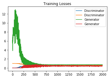
5. Drawing:

fig, ax = plt.subplots()
losses = np.array(ｇ_losses)
plt.plot(d_losses, label='Discriminator')
plt.plot(g_losses, label='Generator')
plt.title("Training Losses")
plt.legend()