Article catalog
Kingma D P, Ba J. Adam: A Method for Stochastic Optimization[J]. arXiv: Learning, 2014.
@article{kingma2014adam:,
title={Adam: A Method for Stochastic Optimization},
author={Kingma, Diederik P and Ba, Jimmy},
journal={arXiv: Learning},
year={2014}}
General
a great reputation.
primary coverage
F (theta) f (theta) f (theta) is used to represent the objective function. The stochastic optimization usually needs to minimize e (f (theta)) \ matchb {e} (f(\ theta)) e (f (theta)), but because we take a small batch every time, we actually deal with F1 (theta) ,ft(θ)f_1(\theta),\ldots, f_T(\theta)f1(θ),… , ft (θ). Use gt = ∇ θ ft (θ) g_ t=\nabla_ {\theta}f_ T (theta) gt = ∧ ft (θ) represents the gradient corresponding to step ttt
Adam method estimates gradient e (GT) and mathbb {e} (g) respectively_ t) The origin of the first and second moments of E (GT)
algorithm
Note: the following algorithms are all element wise operations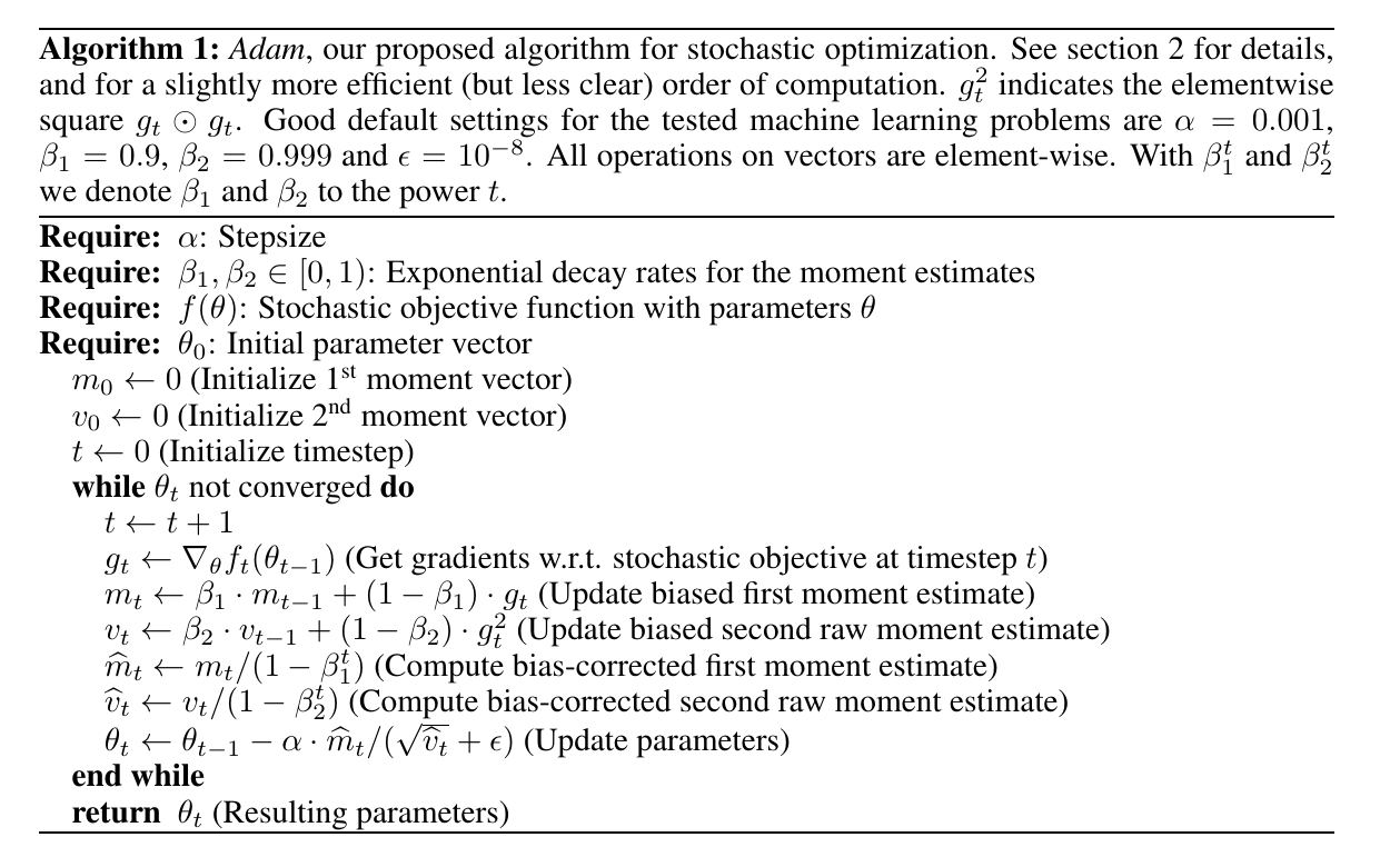
Select appropriate parameters
First, analyze why there are
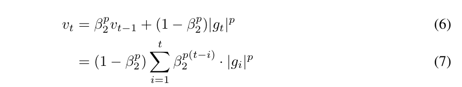
m^t←mt/(1−β2t),v^t←vt/(1−β2t).(A.1)
\tag{A.1}
\hat{m}_t \leftarrow m_t / (1-\beta_2^t), \\
\hat{v}_t \leftarrow v_t / (1-\beta_2^t).
m^t←mt/(1−β2t),v^t←vt/(1−β2t).(A.1)
Can be proved by induction
mt=(1−β1)∑i=1tβ1t−i⋅givt=(1−β2)∑i=1tβ2t−i⋅gi2.(A.2)
\tag{A.2}
m_t = (1-\beta_1) \sum_{i=1}^t \beta_1^{t-i} \cdot g_i \\
v_t = (1-\beta_2) \sum_{i=1}^t \beta_2^{t-i} \cdot g_i^2.
mt=(1−β1)i=1∑tβ1t−i⋅givt=(1−β2)i=1∑tβ2t−i⋅gi2.(A.2)
If the distribution is stable: E[gt]=E[g],E[gt2]=E[g2]\mathbb{E}[g_t]=\mathbb{E}[g],\mathbb{E}[g_t^2]=\mathbb{E}[g^2]E[gt] = E [g], E [G T 2] = E[g2], then
E[mt]=E[g]⋅(1−β1t)E[vt]=E[g2]⋅(1−β2t).(A.3)
\tag{A.3}
\mathbb{E}[m_t]=\mathbb{E}[g] \cdot(1-\beta_1^t) \\
\mathbb{E}[v_t]= \mathbb{E}[g^2] \cdot (1- \beta_2^t).
E[mt]=E[g]⋅(1−β1t)E[vt]=E[g2]⋅(1−β2t).(A.3)
That's why there is (A.1) this step
A large application scenario when Adam proposed is dropout, which often requires us to take a larger β 2\beta_2 β 2 (it can be understood as offsetting random factors)
Since E[g]/E[g2] < 1 \ mathb {e} [g] / \ sqrt {\ mathb {e} [G ^ 2]} \ Le 1E[g]/E[g2] < 1, we can understand step α as a trust region (since ∣ Δ t ∣ < a | De lt a_ t| \frac{<}{\approx} a∣Δt∣≈<a).
Another important property is that, for example, the function expands (or shrinks) ccc times cfcf, and the gradient is cgcgcg, which corresponds to
c⋅m^tc2⋅v^t=m^tv^t,
\frac{c \cdot \hat{m}_t}{\sqrt{c^2 \cdot \hat{v}_t}}= \frac{\hat{m}_t}{\sqrt{\hat{v}_t}},
c2⋅v^tc⋅m^t=v^tm^t,
There is no change
Some other optimization algorithms
AdaGrad:
θt+1=θt−α⋅1∑i=1tgt2+ϵgt. \theta_{t+1} = \theta_t -\alpha \cdot \frac{1}{\sqrt{\sum_{i=1}^tg_t^2}+\epsilon} g_t. θt+1=θt−α⋅∑i=1tgt2+ϵ1gt.
RMSprop:
vt=β2vt−1+(1−β2)gt2θt+1=θt−α⋅1vt+ϵgt. v_t = \beta_2 v_{t-1} + (1-\beta_2) g_t^2 \\ \theta_{t+1} = \theta_t -\alpha \cdot \frac{1}{\sqrt{v_t+\epsilon}}g_t. vt=β2vt−1+(1−β2)gt2θt+1=θt−α⋅vt+ϵ1gt.
AdaDelta:
vt=β2vt−1+(1−β2)gt2θt+1=θt−α⋅mt−1+ϵvt+ϵgtmt=β1mt−1+(1−β1)[θt+1−θt]2. v_t = \beta_2 v_{t-1} + (1-\beta_2) g_t^2 \\ \theta_{t+1} = \theta_t -\alpha \cdot \frac{\sqrt{m_{t-1}+\epsilon}}{\sqrt{v_t+\epsilon}}g_t \\ m_t = \beta_1 m_{t-1}+(1-\beta_1)[\theta_{t+1}-\theta_t]^2. vt=β2vt−1+(1−β2)gt2θt+1=θt−α⋅vt+ϵmt−1+ϵgtmt=β1mt−1+(1−β1)[θt+1−θt]2.
Note: item by item
AdaMax
Another algorithm is proposed in this paper
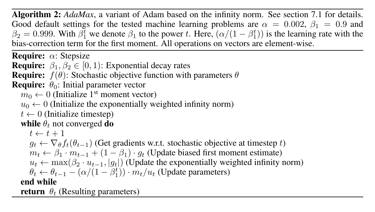
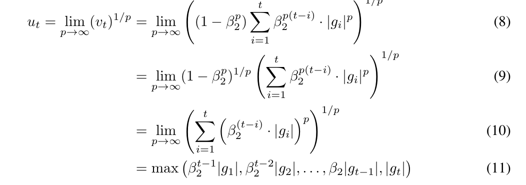

theory
I don't want to talk about it. I feel that there are many mistakes
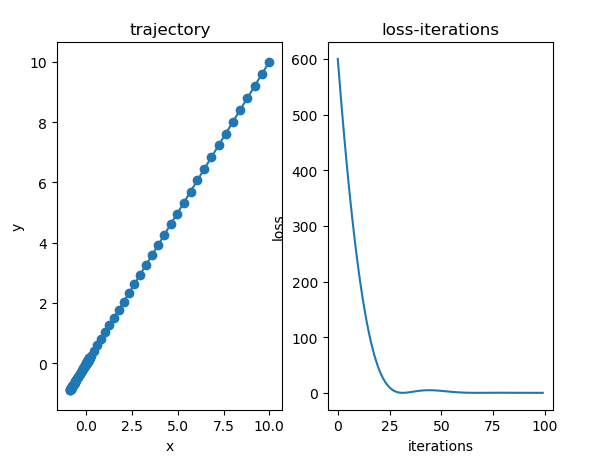
code
import numpy as np

class Adam:

    def __init__(self, instance, alpha=0.001, beta1=0.9, beta2=0.999,
                 epsilon=1e-8, beta_decay=1., alpha_decay=False):
        """ the Adam using numpy
        :param instance: the theta in paper, should have the grad method to call the grads
                            and the zero_grad method for clearing the grads
        :param alpha: the same as the paper default:0.001
        :param beta1: the same as the paper default:0.9
        :param beta2: the same as the paper default:0.999
        :param epsilon: the same as the paper default:1e-8
        :param beta_decay:
        :param alpha_decay: default False, if True, we will set alpha = alpha / sqrt(t)
        """
        self.instance = instance
        self.alpha = alpha
        self.beta1 = beta1
        self.beta2 = beta2
        self.epsilon = epsilon
        self.beta_decay = beta_decay
        self.alpha_decay = alpha_decay
        self.initialize_paras()

    def initialize_paras(self):
        self.m = 0.
        self.v = 0.
        self.timestep = 0

    def update_paras(self):
        grads = self.instance.grad
        self.beta1 *= self.beta_decay
        self.beta2 *= self.beta_decay
        self.m = self.beta1 * self.m + (1 - self.beta1) * grads
        self.v = self.beta2 * self.v + (1 - self.beta2) * grads ** 2
        self.timestep += 1
        if self.alpha_decay:
            return self.alpha / np.sqrt(self.timestep)
        return self.alpha

    def zero_grad(self):
        self.instance.zero_grad()

    def step(self):
        alpha = self.update_paras()
        betat1 = 1 - self.beta1 ** self.timestep
        betat2 = 1 - self.beta2 ** self.timestep
        temp = alpha * np.sqrt(betat2) / betat1
        self.instance.parameters -= temp * self.m / (np.sqrt(self.v) + self.epsilon)


class PPP:

    def __init__(self, parameters, grad_func):
        self.parameters = parameters
        self.zero_grad()
        self.grad_func = grad_func

    def zero_grad(self):
        self.grad = np.zeros_like(self.parameters)

    def calc_grad(self):
        self.grad += self.grad_func(self.parameters)


def f(x):
    return x[0] ** 2 + 5 * x[1] ** 2

def grad(x):
    return np.array([2 * x[0], 100 * x[1]])


if __name__ == "__main__":

    x = np.array([10., 10.])
    x = PPP(x, grad)
    xs = []
    ys = []
    optim = Adam(x, alpha=0.4)
    for i in range(100):
        xs.append(x.parameters.copy())
        y = f(x.parameters)
        ys.append(y)
        optim.zero_grad()
        x.calc_grad()
        optim.step()
    xs = np.array(xs)
    ys = np.array(ys)
    import matplotlib.pyplot as plt
    fig, (ax0, ax1)= plt.subplots(1, 2)
    ax0.plot(xs[:, 0], xs[:, 1])
    ax0.scatter(xs[:, 0], xs[:, 1])
    ax0.set(title="trajectory", xlabel="x", ylabel="y")
    ax1.plot(np.arange(len(ys)), ys)
    ax1.set(title="loss-iterations", xlabel="iterations", ylabel="loss")
    plt.show()