Recently, pytorch has been used in the group report, so I want to organize the relevant content into a blog (report ppt and demonstration code are attached at the end, you can take them if necessary). It mainly refers to the previous chapters of Python deep learning: Based on pytorch and some online introductory tutorials, focusing on code. Through this blog, you can:

1. Have a preliminary understanding of PyTorch framework

2. Have a certain understanding of Tensor tensor, autograd automatic derivation, back propagation and other concepts in PyTorch and master relevant codes

3. Implement a simple machine learning algorithm (function fitting) with PyTorch

4. Using PyTorch neural network toolbox to build a simple convolution neural network model (minist handwritten digit recognition)

5. Train the constructed network and predict through the model
   ...

1, PyTorch introduction

1.1 introduction to pytorch

PyTorch comes from the deep learning framework, Torch, which uses Lua, a language that is not very popular, as an interface, and not many people use it. Therefore, the development team rewrites a new deep learning framework, PyTorch, based on the Torch using Python.
Although the predecessor of PyTorch is Torch, the difference between PyTorch and Torch is that PyTorch is not only more flexible and supports dynamic graph, but also provides Python interface. PyTorch can be seen as a numpy with GPU support, and also as a powerful deep neural network with automatic derivation function. It is more like the substitute product of numpy. It not only inherits many advantages of numpy, but also supports GPU computing, and has more obvious advantages in computing efficiency than numpy. Moreover, PyTorch has many advanced functions, such as rich API, which can quickly complete the construction and training of deep neural network model. So as soon as PyTorch is released, it is sought after and loved by many developers and researchers, and becomes one of the important tools for AI practitioners.

1.2 advantages of pytorch

• concise
  PyTorch pursues the least encapsulation and avoids making wheels repeatedly, unlike tensor flow, which is full of session, graph, operation and name_scope, variable, sensor, layer and other new concepts
  PyTorch is designed to represent high-dimensional array (sensor), variable\autograd and neural network( nn.Module )There are three levels of abstraction from low to high, and the three abstractions are closely related, which can be modified and operated at the same time nn.Module The encapsulation of all model objects in PyTorch
• Easy to use
  The current deep learning platform mainly uses two ways to define the model: static calculation graph and dynamic calculation graph. Most platforms adopt the static definition method, including TensorFlow, Theano, Caffe, Keras, etc
  Static graph needs to define a complete set of model before processing data, while dynamic graph model allows users to define a basic framework first and then modify the model in real time according to the data
  The defect of static graph definition is that a complete set of models must be defined before data processing, which can handle all marginal situations, for example, the maximum length of sentences in the whole data must be known before model declaration. On the contrary, dynamic graph models (such as PyTorch, Chainer, Dynet) can define models very freely
  PyTorch is not only simple in defining network structure, but also intuitive and flexible. It supports autograd, so it doesn't need to define and deduce back-propagation by itself. It also supports dynamic graph model, which can seamlessly connect numpy
• Fast
  PyTorch's flexibility does not come at the cost of speed. In many reviews, PyTorch outperforms frameworks such as TensorFlow and Keras. In the same algorithm, the implementation with PyTorch is more likely to be faster than that with other frameworks
• Community activity
  PyTorch provides complete documents, with the strong support of facebook's FAIR (FAIR is the world's top 3 AI research institution), and many open-source solutions

1.3 installation of pytorch

Main process:

1. Create python environment in anaconda and add path to system environment variable
2. Copy the installation command on the pytorch official website https://pytorch.org/get-started/locally/
3. Installing pytorch on the command line
4. Import torch test whether the installation is successful

Please refer to blog for details https://blog.csdn.net/qq_38704904/article/details/95192856

2, PyTorch Foundation

2.1 Numpy

NumPy is an extension library of Python language, which supports a large number of dimensional array and matrix operations. In addition, NumPy also provides a large number of mathematical function libraries for array operations, which are often used in machine learning and deep learning.

2.1.1 definition of numpy array

• Direct definition

import numpy as np
x1 = np.array([1.0, 2.0, 3.0])
X2=np.array((1.0, 2.0, 3.0))

• Convert list list to numpy array

b=[2.0,4.0,6.0]
y=np.array(a)

• Convert numpy array to list

z= np.array([1.0, 2.0, 3.0]) 
c=list(z)

2.1.2 element access of numpy array

For matrix A=np.array([1,2,3],[4,5,6])

• A[i] obtains row I of matrix A
• A[i][j] obtains the element Aij
• A[i][j:k] gets the j to k-1 elements of array A[i]

2.1.3 calculation of numpy array

• Add: x+y
• Multiplication: x*y
• Broadcast: x*10=[1.0, 2.0, 3.0]10=[1.0, 2.0, 3.0] [10, 10, 10]

2.2 Tensors tensor

2.2.1 Tensors

2.2.2 use of tensors

1. Import package

import torch

1. Build a 5 * 3 matrix

x = torch.Tensor(5, 3)  # uninitialized
y = torch.rand(5, 3)  # Random initialization

1. Convert torch's Tensor to numpy's array

a=x.numpy() # Tensor to array
x=torch.from_numpy(a)  # array to Tensor

1. Operation:

• Addition and subtraction: y.add_(x),z=x+y, torch.add(x,y,out=z),z=torch.sub(x,y)
• Multiplication: x*y torch.mul(x,y)
• Crop: y=torch.clamp(x,-0.1,0.1)
  For more operations, please refer to Official documents

1. CUDA Tensors:
   Use the. cuda function to move Tensors to GPU

if torch.cuda.is_available():
    x = x.cuda()
    y = y.cuda()

2.3 automatic derivation of autograd

2.3.1 Variable
After the Tensor is converted to Variable, the gradient information can be loaded. Once the forward calculation is performed, all gradients can be automatically calculated by the. backward() method

2.3.2 gradient descent
The gradient of the loss function with respect to the parameters of the model points to a direction that can reduce the value of the loss function, and the model can be continuously updated along the gradient direction to minimize the loss function

2.3.3 auto derivative
For complex models, such as neural networks with dozens of layers, it is very difficult to calculate the gradient manually. Therefore, PyTorch provides an Autograd package to automate the derivation process. It will have a recorder to record all our operations, and then play back the records to calculate the gradient
This technique is particularly effective in building neural networks, because we can save time by calculating the differential of the front parameters

2.4 function fitting with Numpy

import numpy as np
from matplotlib import pyplot as plt
# Generate input data x and target data y
np.random.seed(100)
x = np.linspace(-1,1,100).reshape(100,1)
y = 3*np.power(x,2)+2+0.2*np.random.rand(x.size).reshape(100,1)
# View the distribution of x and y data
plt.scatter(x,y)
plt.show()
# Initialize weight parameters
w1 = np.random.rand(1,1)
b1 = np.random.rand(1,1)
# Training model
lr = 0.001 # Learning rate
for i in range(800): #gradient descent 
    y_pred = np.power(x,2)*w1+b1

    loss = 0.5*(y_pred - y)**2  # loss function 
    loss = loss.sum()  # variance
    # Gradient descent method
    grad_w = np.sum((y_pred - y)*np.power(x,2))
    grad_b = np.sum((y_pred - y))
    w1 -= lr*grad_w  # Consider learning rate as step size
    b1 -= lr*grad_b
# Visualization results
plt.plot(x,y_pred,'r-',label='predict')
plt.scatter(x,y,color='blue',marker='o',label='true') # true data
plt.xlim(-1,1)
plt.ylim(2,6)
plt.legend()
plt.show()
print(w1,b1)

Set the objective function to y_pred=w1 * x^2+b1, solving the objective function is equivalent to solving the parameters w1 and b1
The loss function defined here is 0.5 * (Y_ The sum of PRED - y) ^ 2 is equal to the variance (according to the video of Wu Enda, multiplying by 0.5 can easily eliminate the coefficient of the second power when deriving, so the actual multiplied by 0.5). The smaller the value of the loss function is, the smaller the error will be, so it is equivalent to solving the w1 and b1 that make the minimum loss value, so the objective function is the closest to the actual function.
grad_w is the gradient of W 1, which is the derivative of loss to w 1, grad_b is the gradient of b1, which is equivalent to the partial derivative of loss to b1. Along the gradient direction, B can reach the lowest point of loss as soon as possible.
Note that the gradient here is calculated manually by ourselves, about this process: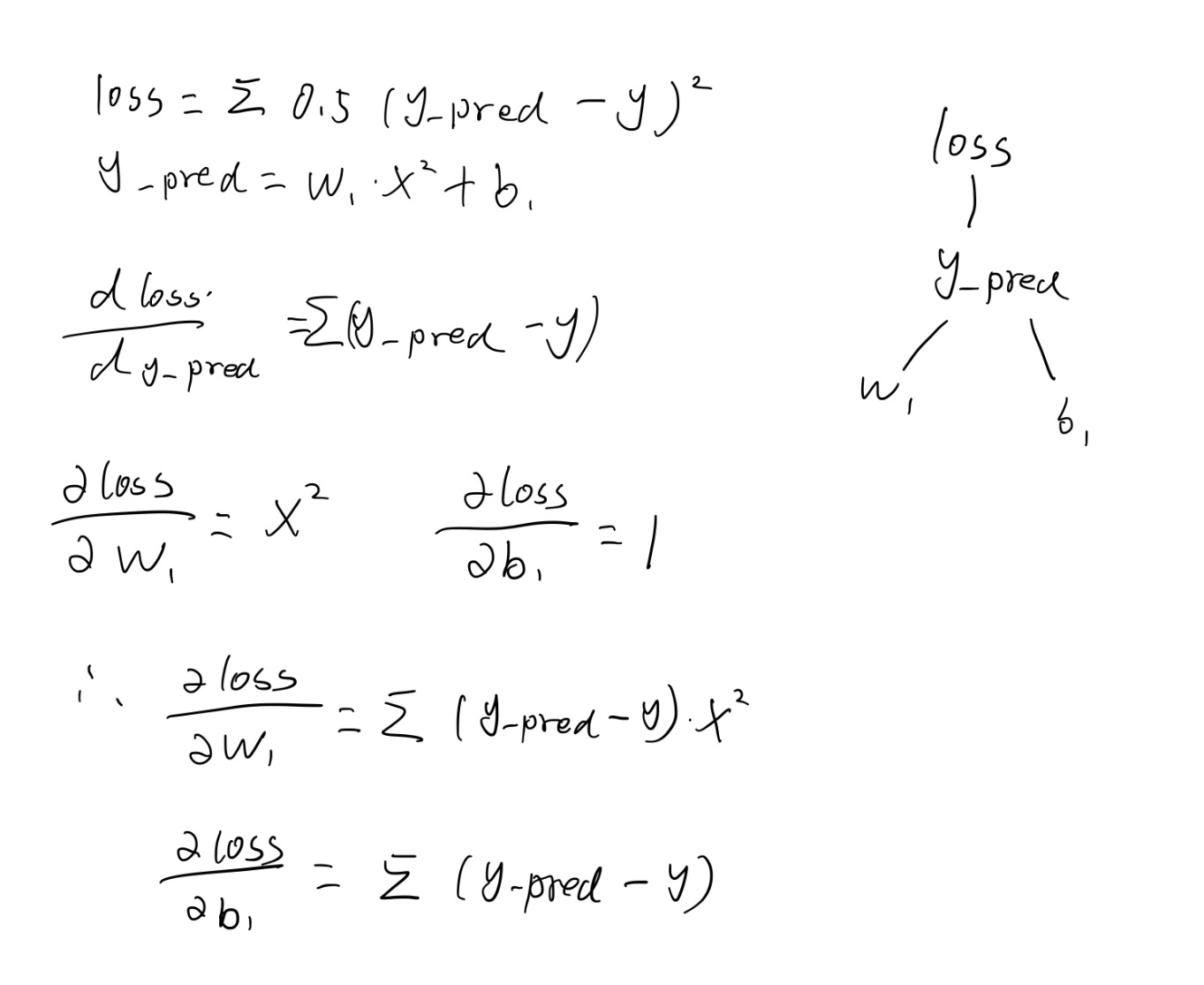

therefore

    grad_w = np.sum((y_pred - y)*np.power(x,2))
    grad_b = np.sum((y_pred - y))

Then let w1 and b1 move a small step along the gradient direction each time, so that the gradient of w1 and w2 will be smaller and smaller, and when it is close to 0, the possible minimum value of loss will be obtained

    w1 -= lr*grad_w  # Consider learning rate as step size
    b1 -= lr*grad_b

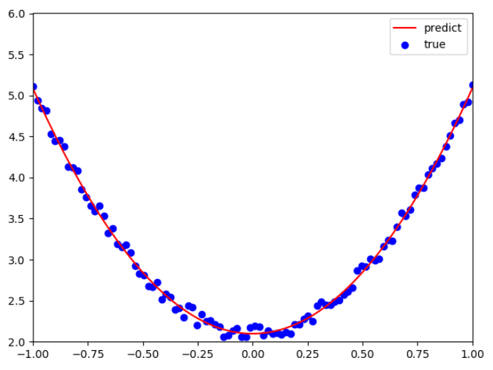
Cycle the calculation 800 times, output the updated w1 and b1, and output the fitting image
Operation result: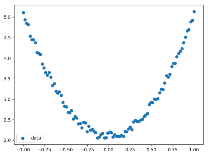



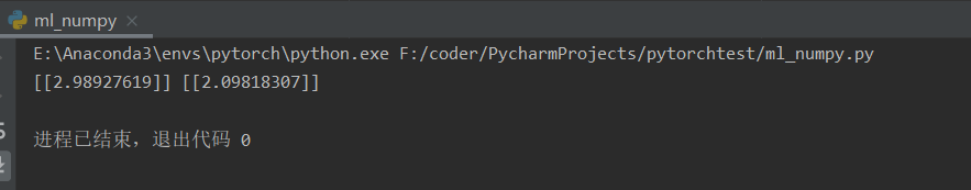
It can be concluded that w1=2.98927619, b1=2.09818307, and the objective function y_pred=2.98927619x^2+2.09818307.

2.5 function fitting with PyTorch

We can see that when the function is simple, it is convenient to calculate the gradient manually, but when the function is complex, the calculation will be very difficult, and the automatic derivation of Python perfectly solves this problem. Just give the forward calculation process, and python will automatically calculate the gradient for you in reverse. Next, take the above case as an example, but use pytorch to realize it.

import numpy as np
import torch
from matplotlib import pyplot as plt
# Generate input data x and target data y
np.random.seed(100)
x = np.linspace(-1,1,100).reshape(100,1)
y = 3*np.power(x,2)+2+0.2*np.random.rand(x.size).reshape(100,1)
x=torch.tensor(x)
y=torch.tensor(y)
# View the distribution of x and y data
plt.scatter(x,y)
plt.show()
# Initialize weight parameters
w1 =torch.zeros(1,1,requires_grad=True)
b1 =torch.zeros(1,1,requires_grad=True)
# Training model
lr = 0.001 # Learning rate
cost = []
for i in range(800): #gradient descent 
    y_pred = w1*x**2 + b1
    loss = torch.sum((y_pred - y) ** 2)
    loss.backward()
    # Parameter update
    print(w1.grad.data.item(),b1.grad.data.item())
    # Gradient descent method
    w1.data = w1.data - lr*w1.grad.data  # Consider learning rate as step size
    b1.data = b1.data - lr*b1.grad.data
    w1.grad.data.zero_()  #Gradient clear
    b1.grad.data.zero_()

# Visualization results
plt.plot(x,y_pred.data,'r-',label='predict')
plt.scatter(x,y,color='blue',marker='o',label='true') # true data
plt.xlim(-1,1)
plt.ylim(2,6)
plt.legend()
plt.show()
print(w1.data,b1.data)

Data and processing process are similar to the previous one, mainly focusing on automatic derivation. First, when defining w1 and w2, w1= torch.zeros (1,1,requires_grad = True), which means that the initial value of sensor w1 in row 1 and column 1 is 0, requires_ The default value of grad is false. If it is True, the gradient needs to be solved

w1 =torch.zeros(1,1,requires_grad=True)
b1 =torch.zeros(1,1,requires_grad=True)

Then we give the original function y_pred=w1 * x^2+b1，loss=Σ0.5*(y_ PRED - y) after ^ 2 loss.backward(), which represents the backward propagation of loss and the calculation of the partial derivative from loss to W1 and B1. The specific calculation process of the machine can be referred to Calculation chart and automatic derivation In this way, it is not necessary to manually calculate the corresponding gradient formula, directly W1 grad.data.item () get the value of gradient (w1.grad can get gradient, but the result is a sensor variable)
Note that it is necessary to clear the gradient in each cycle, otherwise the gradient in front of each cycle will be accumulated, and the larger the calculation is, it is contrary to the purpose of gradient descent

w1.grad.data.zero_()  #Gradient clear

3, PyTorch neural network toolbox

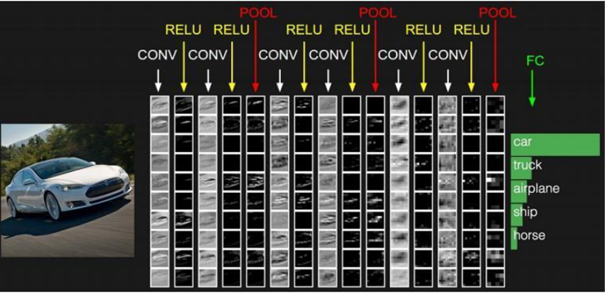
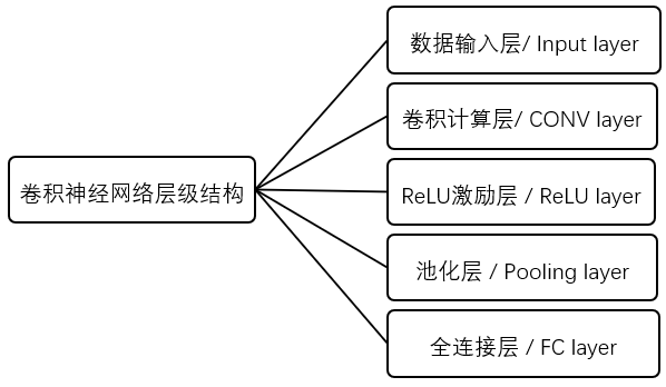
3.1 convolution neural network level

Convolution neural network is a kind of feedforward neural network which contains convolution operation and has deep hierarchy structure. The difference between convolution neural network and traditional neural network is that the layer and form of convolution neural network have changed a lot, which can be said to be an improvement of traditional neural network. As shown in the figure below, the traditional neural network mainly includes an input layer, an output layer and several intermediate layers, while the convolutional neural network has many layers that the traditional neural network does not have.

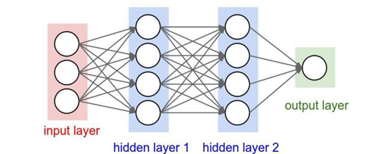
The input layer is the large amount of training data that you feed in, so it mainly introduces the implementation of pytorch to other layers:

3.1.1 convolution

Convolution computing layer is the core layer of convolution neural network, which consists of several convolution units. In this convolution layer, there are two key operations, one is local correlation, which regards each neuron as a filter, the other is window
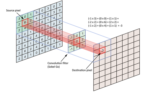
field) to allow the filter to calculate the local data. The convolution calculation layer is composed of several convolution units, each of which is a weight matrix. It will slide a fixed step on the two-dimensional input data every time, and then multiply the element values of the corresponding window by the matrix, and output the calculated results to the pixels.
As shown in Figure 8, it is a convolution calculation operation. The left matrix is the original matrix of the initial input, the middle matrix is the filter, and the right is the output value after convolution calculation. Through convolution operation, different features of input can be extracted and enhanced layer by layer. For example, the first layer of convolution calculation layer may only extract low-level features, while the higher-level network can iteratively extract more complex features from low-level features.

Python implementation:

One dimensional convolution: mostly used for text processing, only width is counted, not height

conv1 = nn.Conv1d(in_channels=256, out_channels=100,
kernel_size=2)
input = torch.randn(32, 35, 256)
input = input.permute(0, 2, 1)
output = conv1(input)

Two dimensional convolution: mostly used for image processing

from PIL import Image
from torchvision.transforms
import ToTensor, ToPILImage
to_tensor = ToTensor()  # img ->tensor
to_pil = ToPILImage()  # tensor -> image
ll =Image.open('imgs/lena.png')  
input =to_tensor(lena).unsqueeze(0) 

3.1.2 activation layer

If the activation function is added to the neural network, the nonlinear factors can be introduced, the expression intensity of the model can be improved, the training time of the model can be reduced, the training cost can be reduced, and many problems that cannot be solved by the linear model can be solved.

Python implements the relu function: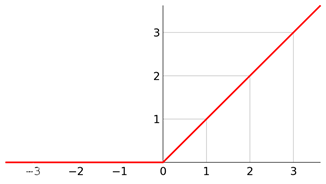

relu = nn.ReLU(inplace=True)
output = relu(input)
# output = input.clamp(min=0)

3.1.3 pool layer

In essence, the Pooling layer is a sampling operation, while the upsampling is to restore the feature map. Unlike the upsampling, the upsampling is a subsampling operation. One is to compress the amount of data, that is, to compress the input feature image to reduce the image size to achieve the purpose of reducing the required display memory; the other is to compress the feature image Map becomes smaller, that is to say, the feature value in the compressed input image features reduces the amount of calculation, removes redundant information in the feature value to retain the most important features, and improves the over fitting situation.

Common pooling operations include average
Pooling and max pooling Pooling), in which the average value of the image area is taken as the value after pooling the area. The average pool can keep the background well, but it will make the image fuzzy. The maximum pool is to select the maximum value of the image area as the value after pooling the area, which can better retain the image texture features. Generally speaking, the maximum pool is more commonly used than the average pool .

Average pooling: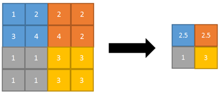

Maximum pooling: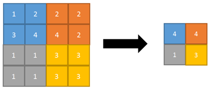

Python implementation:

pool1= nn.AvgPool2d(2,2)  # Average pooling
pool2= nn. MaxPool2d(2,2)  # Maximum pooling
out   = pool1( V(input) )
out   = pool2( V(input) )

3.1.4 full connection layer (output layer)

In the convolution neural network, there will be one or more full connection layers at the tail of convolution neural network after several convolution layers and pooling layers. It is mainly responsible for the full connection with all neurons in the upper layer, integrating the local features obtained in the convolution layer and pooling layer to get the final feature image.

Python implementation:

input = V(t.randn(2,3))
linear = nn.Linear(3,4)
h = linear(input)

3.2 building convolutional neural network with pytorch

Next, take mnist handwritten digit recognition as an example to build a simple convolutional neural network model using PyTorch neural network toolbox (the complete code is at the end)

Get the training data set first

# Get training set dataset
training_data = torchvision.datasets.MNIST(
    root='./data/',  # dataset storage path
    train=True,  # True means train training set, False means test test test set   
    transform=torchvision.transforms.ToTensor(),  # Normalize the original data to (0,1) interval
    download=DOWNLOAD_MNIST,
)

# Size of training set and test set for printing MNIST data set
print(training_data.data.size())   # torch.Size([60000, 28, 28])
print(training_data.targets.size())   # torch.Size([60000])
# Print one to see what it looks like
plt.imshow(training_data.data[0].numpy(), cmap='gray')
plt.title('simple')
plt.show()

#adopt torchvision.datasets The acquired dataset format can be directly placed in DataLoader
train_loader = Data.DataLoader(dataset=training_data,
batch_size=BATCH_SIZE,shuffle=True)

# Get test set dataset
test_data = torchvision.datasets.MNIST(root='./data/',train=False)

# Take the first 2000 test set samples
test_x = Variable(torch.unsqueeze(test_data.data, dim=1),volatile=True).type(torch.FloatTensor)[:2000] / 255
# (2000, 28, 28) to (2000, 1, 28, 28), in range(0,1)
test_y = test_data.targets[:2000]

This is the data set of pytorch. The picture looks like this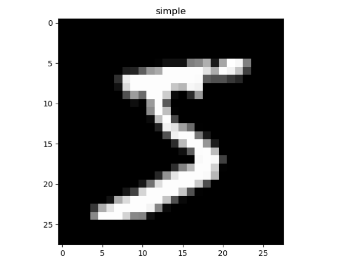
If you don't have a mnist dataset, it will automatically download it to you, but the download will be slow, so you can create a new data directory after downloading, and then put the downloaded dataset in, saving time

Link: https://pan.baidu.com/s/1TlvwqzkvfICdAceHITcMyw
Extraction code: u0nk

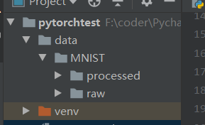
You can see that there are two directories in MNIST: processed and raw. Processed is used to put the training files generated in the training process, which is not very controlled, while raw is used to store the training pictures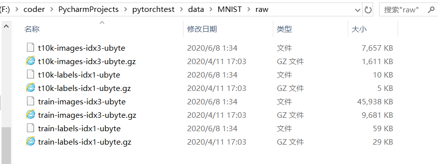

Then the structure of cnn is designed, and a convolutional neural network with the following structure is defined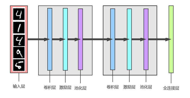

class CNN(nn.Module):
    def __init__(self):
        super(CNN, self).__init__()
        self.conv1 = nn.Sequential(  # (1,28,28)
            nn.Conv2d(in_channels=1, out_channels=16, kernel_size=5,
                      stride=1, padding=2),  # (16,28,28)
            # The size of the image you want to convolute from con2d does not change, padding=(kernel_size-1)/2
            nn.ReLU(),
            nn.MaxPool2d(kernel_size=2)  # (16,14,14)
        )
        self.conv2 = nn.Sequential(  # (16,14,14)
            nn.Conv2d(16, 32, 5, 1, 2),  # (32,14,14)
            nn.ReLU(),
            nn.MaxPool2d(2)  # (32,7,7)
        )
        self.out = nn.Linear(32 * 7 * 7, 10)

    def forward(self, x):
        x = self.conv1(x)
        x = self.conv2(x)
        x = x.view(x.size(0), -1)  # Flatten (batch, 32, 7, 7) to (batch, 32 * 7 * 7)
        output = self.out(x)
        return output

Take a closer look at the overall structure of cnn defined:

CNN(
(conv1): Sequential(
(0): Conv2d(1, 16, kernel_size=(5, 5), stride=(1, 1), padding=(2, 2))
(1): ReLU()
(2): MaxPool2d(kernel_size=2, stride=2, padding=0, dilation=1, ceil_mode=False)
)
(conv2): Sequential(
(0): Conv2d(16, 32, kernel_size=(5, 5), stride=(1, 1), padding=(2, 2))
(1): ReLU()
(2): MaxPool2d(kernel_size=2, stride=2, padding=0, dilation=1, ceil_mode=False)
)
(out): Linear(in_features=1568, out_features=10, bias=True)
)

There are two parts in total -- conv1 and conv2

conv1 includes a two-dimensional convolution layer:

nn.Conv2d(in_channels=1, out_channels=16, kernel_size=5,
                      stride=1, padding=2),  # (16,28,28)

An incentive layer:

nn.ReLU()

An average pool layer:

nn.MaxPool2d(kernel_size=2)

The same is true for conv2.
Finally, it is a full connection layer, or an output layer

self.out = nn.Linear(32 * 7 * 7, 10)

forward is the original calculation process, which can be used for back propagation later

def forward(self, x):
    x = self.conv1(x)
    x = self.conv2(x)
    x = x.view(x.size(0), -1)  # Flatten (batch, 32, 7, 7) to (batch, 32 * 7 * 7)
    output = self.out(x)
    return output

The X here is equivalent to the input layer. First put x into the first conv1 (convolution excitation pooling), then put the output structure into the second conv2 (convolution excitation pooling), then put it into the output layer out, and finally return the output result

3.3 model training and prediction

Train the constructed network and predict it through the model

First instantiate the cnn network cnn = CNN() just designed, and then set an Adam optimizer for optimization

optimizer = torch.optim.Adam(cnn.parameters(), lr=LR)
loss_function = nn.CrossEntropyLoss()

Cycle training

for epoch in range(EPOCH):
    for step, (x, y) in enumerate(train_loader):
        b_x = Variable(x)
        b_y = Variable(y)

        output = cnn(b_x)
        loss = loss_function(output, b_y)  #loss function 
        optimizer.zero_grad()   
        loss.backward()
        optimizer.step()

        if step % 100 == 0:
            test_output = cnn(test_x)
            pred_y = torch.max(test_output, 1)[1].data.squeeze()
            s1=sum(pred_y == test_y)
            s2=test_y.size(0)
            accuracy = s1/(s2*1.0)
            print('Epoch:', epoch, '|Step:', step,
                  '|train loss:%.4f' % loss.item(), '|test accuracy:%.4f' % accuracy)

among optimizer.zero_grad() is to clear the previous gradient, then call backward() on loss, and finally, call optimizer.step() add the updated value to the parameters of the model.
About optimizer( torch.optim )Use of

Output the current loss value and accuracy every 100 times of training, where accuracy = the total number / total number of prediction results and correct results are the same

Epoch: 0 |Step: 0 |train loss:2.3105 |test accuracy:0.0605
Epoch: 0 |Step: 100 |train loss:0.1290 |test accuracy:0.8735
Epoch: 0 |Step: 200 |train loss:0.4058 |test accuracy:0.9285
Epoch: 0 |Step: 300 |train loss:0.1956 |test accuracy:0.9440
Epoch: 0 |Step: 400 |train loss:0.1238 |test accuracy:0.9585
Epoch: 0 |Step: 500 |train loss:0.2217 |test accuracy:0.9630
Epoch: 0 |Step: 600 |train loss:0.0237 |test accuracy:0.9670
Epoch: 0 |Step: 700 |train loss:0.2158 |test accuracy:0.9700
Epoch: 0 |Step: 800 |train loss:0.0433 |test accuracy:0.9720
Epoch: 0 |Step: 900 |train loss:0.0564 |test accuracy:0.9770
Epoch: 0 |Step: 1000 |train loss:0.0320 |test accuracy:0.9760
Epoch: 0 |Step: 1100 |train loss:0.0233 |test accuracy:0.9825

It can be seen that the gradient is decreasing and the accuracy is increasing.

Then use the trained model to predict

test_output = cnn(test_x[:10])
pred_y = torch.max(test_output, 1)[1].data.numpy().squeeze()
print(pred_y, 'prediction number')
print(test_y[:10].numpy(), 'real number')

for n in range(10):
    plt.imshow(test_data.data[n].numpy(), cmap='gray')
    plt.title('data[%i' % n+']:   test:%i' % test_data.targets[n]+'   pred:%i' % pred_y[n])
    plt.show()

Take out the first 10 pictures in the test set and put them into the trained network for test_output = cnn(test_x[:10]) (other parts can also be cut) to obtain the predicted value pred_y = torch.max(test_output, 1)[1].data.numpy().squeeze(), and then output the predicted values and actual labels of these 10 pictures

It can also be displayed in the image plt.imshow(test_data.data[n].numpy(), cmap='gray')

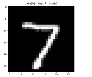
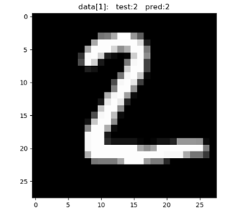
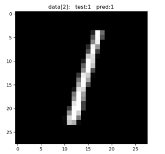
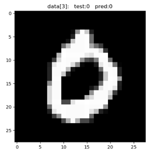
It can be seen that the recognition is quite accurate.

Attachment: complete code of handwritten digit recognition:

import torch
import torch.nn as nn
from torch.autograd import Variable
import torch.utils.data as Data
import torchvision
import matplotlib.pyplot as plt

torch.manual_seed(1)

EPOCH = 1
BATCH_SIZE = 50
LR = 0.001
DOWNLOAD_MNIST = True

# Get training set dataset
training_data = torchvision.datasets.MNIST(
    root='./data/',  # dataset storage path
    train=True,  # True means train training set, False means test test test set
    transform=torchvision.transforms.ToTensor(),  # Normalize the original data to (0,1) interval
    download=DOWNLOAD_MNIST,
)

# Size of training set and test set for printing MNIST data set
print(training_data.data.size())
print(training_data.targets.size())
# torch.Size([60000, 28, 28])
# torch.Size([60000])
plt.imshow(training_data.data[0].numpy(), cmap='gray')
plt.title('simple')
plt.show()

# adopt torchvision.datasets The acquired dataset format can be directly placed in DataLoader
train_loader = Data.DataLoader(dataset=training_data, batch_size=BATCH_SIZE,
                               shuffle=True)

# Get test set dataset
test_data = torchvision.datasets.MNIST(root='./data/', train=False)
# Take the first 2000 test set samples

test_x = Variable(torch.unsqueeze(test_data.data, dim=1),
                  volatile=True).type(torch.FloatTensor)[:2000] / 255
# (2000, 28, 28) to (2000, 1, 28, 28), in range(0,1)
test_y = test_data.targets[:2000]


class CNN(nn.Module):
    def __init__(self):
        super(CNN, self).__init__()
        self.conv1 = nn.Sequential(  # (1,28,28)
            nn.Conv2d(in_channels=1, out_channels=16, kernel_size=5,
                      stride=1, padding=2),  # (16,28,28)
            # The size of the image you want to convolute from con2d does not change, padding=(kernel_size-1)/2
            nn.ReLU(),
            nn.MaxPool2d(kernel_size=2)  # (16,14,14)
        )
        self.conv2 = nn.Sequential(  # (16,14,14)
            nn.Conv2d(16, 32, 5, 1, 2),  # (32,14,14)
            nn.ReLU(),
            nn.MaxPool2d(2)  # (32,7,7)
        )
        self.out = nn.Linear(32 * 7 * 7, 10)

    def forward(self, x):
        x = self.conv1(x)
        x = self.conv2(x)
        x = x.view(x.size(0), -1)  # Flatten (batch, 32, 7, 7) to (batch, 32 * 7 * 7)
        output = self.out(x)
        return output


cnn = CNN()
print(cnn)

optimizer = torch.optim.Adam(cnn.parameters(), lr=LR)
loss_function = nn.CrossEntropyLoss()

for epoch in range(EPOCH):
    for step, (x, y) in enumerate(train_loader):
        b_x = Variable(x)
        b_y = Variable(y)

        output = cnn(b_x)
        loss = loss_function(output, b_y)
        optimizer.zero_grad()
        loss.backward()
        optimizer.step()

        if step % 100 == 0:
            test_output = cnn(test_x)
            pred_y = torch.max(test_output, 1)[1].data.squeeze()
            s1=sum(pred_y == test_y)
            s2=test_y.size(0)
            accuracy = s1/(s2*1.0)
            print('Epoch:', epoch, '|Step:', step,
                  '|train loss:%.4f' % loss.item(), '|test accuracy:%.4f' % accuracy)

test_output = cnn(test_x[:10])
pred_y = torch.max(test_output, 1)[1].data.numpy().squeeze()
print(pred_y, 'prediction number')
print(test_y[:10].numpy(), 'real number')

for n in range(10):
    plt.imshow(test_data.data[n].numpy(), cmap='gray')
    plt.title('data[%i' % n+']:   test:%i' % test_data.targets[n]+'   pred:%i' % pred_y[n])
    plt.show()

reference material:

Don't worry about python's CNN implementation
PyTorch deep learning: 60 minute quick start (image classification using CIFAR10 dataset)
An introductory course of deep learning based on PyTorch (4) -- building neural network
Using Numpy, Tensor and Antograd respectively to realize machine learning
Deep learning based on PyTorch

My report ppt and demo code

Link: https://pan.baidu.com/s/1vZUmWc3o6BZw_6B3ArvzlA
Extraction code: k0ap

Link: https://pan.baidu.com/s/1R9R_tYNerfbl71_WMZFS1w
Extraction code: 0rtt

Finally, it's not easy to code. If you have any help, you can give me a compliment and be careful~