Download Data
import os
import tarfile  # Used to compress and decompress files
import urllib

DOWNLOAD_ROOT = "https://raw.githubusercontent.com/ageron/handson-ml/master/"
HOUSING_PATH = "datasets/housing"
HOUSING_URL = DOWNLOAD_ROOT + HOUSING_PATH + "/housing.tgz"


# Download Data
def fetch_housing_data(housing_url=HOUSING_URL, housing_path=HOUSING_PATH):
    if not os.path.isdir(housing_path):
        os.makedirs(housing_path)
    tgz_path = os.path.join(housing_path, "housing.tgz")
    # urlretrieve()Method downloads remote data directly to local location
    urllib.request.urlretrieve(housing_url, tgz_path)
    housing_tgz = tarfile.open(tgz_path)
    housing_tgz.extractall(path=housing_path)  # Unzip the file to the specified path, either to the current path
    housing_tgz.close()
fetch_housing_data()
Loading data
import pandas as pd

def load_housing_data(housing_path=HOUSING_PATH + "/"):
    csv_path = os.path.join(housing_path, "housing.csv")
    return pd.read_csv(csv_path)
housing = load_housing_data()
housing.head()
View data structure
info()
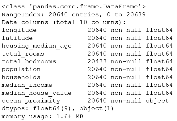
The info() method allows you to quickly see the description of the data, especially the total number of rows, the type of each attribute, and the number of non-null values
housing.describe()
housing.info()
# Analysis: There are 20640 instances in the data set. This is a small amount of data according to machine learning standards, but it is ideal for getting started.
# We noticed that the total number of bedrooms is only 20433 non-empty values, which means that 207 blocks are missing this value.We'll work on it later.
value_counts()
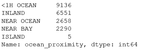
All attributes are numeric except the distance from the sea.It is of type object and can therefore contain any Python object, but since the item is loaded from a CSV file, it must be of type text.When you just looked at the first five items of the data, you may notice that the values in that column are duplicated, meaning that it may be an attribute representing a category.You can use the value_counts() method to see which categories are in the item and how many blocks are in each category:
housing["ocean_proximity"].value_counts()
describe()
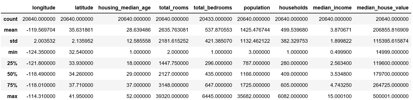
describe() method shows a summary of numeric properties
housing.describe()
Graphic description
Use hist() of matplotlib to draw attribute values as a column chart, which is more intuitive
import matplotlib.pyplot as plt
housing.hist(bins=50, figsize=(10,10))
plt.show() # Not necessary
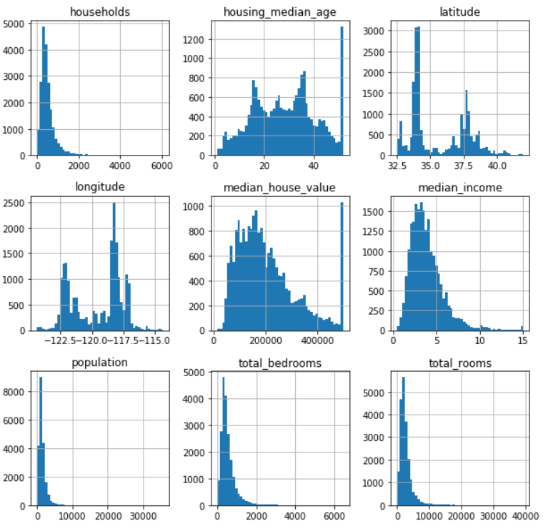
- The median age of a house and the median value of a house are also capped, so there is a straight line at the end of the graph.There are two solutions to this situation
- 1 is to re-collect data that is set to go online
- 2 Remove these data from the training set
- Some columns have long tails that are too far from the median.This makes the detection rule difficult, so later attempts are made to transform the attributes to make them too distributed.
Create Test Set
At this stage, the data will be split.If you look at the test set, you inadvertently choose a specific machine learning model according to the rules in the test set.When you use a test set to assess the error rate, the evaluation is too optimistic and the actual deployed system will perform poorly.This is called perspective bias.
The following three slicing methods:
1. The following method, run the program again, will result in a different test set.One solution is to save the test set from the first run and load it in a subsequent process.Another method is to set the seed of a random number generator (such as np.random.seed(42)) before calling np.random.permutation() to produce a shuffled indices that are always the same
But it's still not perfect
import numpy as np

def split_train_test(data, test_ratio):
    shuffled_indices = np.random.permutation(len(data)) # permutation Chinese Arrangement, Enter Numbers x,take x Random Scattering of Numbers Within
    test_set_size = int(len(data)*test_ratio)
    test_indices = shuffled_indices[:test_set_size]
    train_indices = shuffled_indices[test_set_size:]
    return data.iloc[train_indices], data.iloc[test_indices]

train_set, test_set = split_train_test(housing, 0.2)
print(len(train_set), "train +", len(test_set), "test")
2. Divide by instance's hash value
import hashlib

def test_set_check(identifier, test_ratio, hash):
  return hash(np.int64(identifier)).digest()[-1] < 256 * test_ratio
def split_train_test_by_id(data, test_ratio, id_column, hash=hashlib.md5):
  ids = data[id_column]
  in_test_set = ids.apply(lambda id_: test_set_check(id_, test_ratio, hash))
  return data.loc[~in_test_set], data.loc[in_test_set]

housing_with_id = housing.reset_index() # adds an `index` column
train_set, test_set = split_train_test_by_id(housing_with_id, 0.2, "index")

housing_with_id["id"] = housing["longitude"] * 1000 + housing["latitude"]
train_set, test_set = split_train_test_by_id(housing_with_id, 0.2, "id")
print(len(train_set), "train +", len(test_set), "test")
3.sklearn slicing function
Scikit-Learn provides functions to split datasets into multiple subsets in a variety of ways.The simplest function is `train_test_split', which acts much like the previous function `split_train_test', with a few other functions.For example, it has a `random_state'parameter that allows you to set the random generator seed as described earlier.
from sklearn.model_selection import train_test_split

train_set, test_set = train_test_split(housing, test_size=0.2, random_state=42)
print(len(train_set), "train +", len(test_set), "test")
sklearn slicing function 2
train_test_split is pure random sampling and is suitable for large sample sizes.However, if the dataset is small, there is a risk of sampling bias.Layered sampling is performed.You can use Scikit-Learn's StratfiedShuffleSplit class
housing["income_cat"] = np.ceil(housing["median_income"] / 1.5) # ceil Rounding off values (to produce discrete classifications) divided by 1.5 To limit the number of income classifications
housing["income_cat"].where(housing["income_cat"] < 5, 5.0, inplace=True) # Categorize all categories in 5 into Category 5

from sklearn.model_selection import StratifiedShuffleSplit

split = StratifiedShuffleSplit(n_splits=1, test_size=0.2, random_state=42)

for train_index, test_index in split.split(housing, housing["income_cat"]):
  strat_train_set = housing.loc[train_index]
  strat_test_set = housing.loc[test_index]

# Remember to cull`income_cat`attribute
for set in (strat_train_set, strat_test_set):
  set.drop(["income_cat"], axis=1, inplace=True)
Data exploration, visualization and discovery
Now that you've looked at the data, you need to understand it.
Only study the training set. If the training set is very large, you will need to develop another exploration set to speed up the operation.(Not needed for this example)
Create a copy to avoid damaging the training set
housing = strat_train_set.copy()
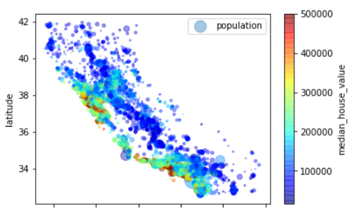
Geographic Data Visualization
housing.plot(kind="scatter", x="longitude", y="latitude", alpha=0.4, s=housing["population"]/100, label="population",
 c="median_house_value", cmap=plt.get_cmap("jet"), colorbar=True,)
# The radius of each circle represents the population of the block (option)`s`),Color represents price (option)`c`)
plt.legend()
Find Associations
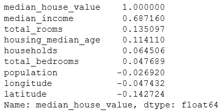
Correlation coefficient 1
When the dataset is not very large, it is easy to calculate the standard correlation coefficient (also known as Pearson correlation coefficient) between each pair of attributes using the corr() method.
corr_matrix = housing.corr()
corr_matrix["median_house_value"].sort_values(ascending=False)
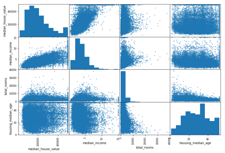
Coefficient of correlation 2
attributes = ["median_house_value", "median_income", "total_rooms",
 "housing_median_age"]
pd.plotting.scatter_matrix(housing[attributes], figsize=(12, 8))
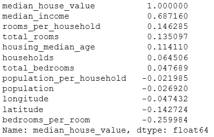
Attribute Combination Experiment
Some attributes are not useful by themselves, but when combined with other attributes.For example, the number of rooms below and the number of homeowners themselves are not useful, and the number of rooms per household is more useful when divided.So in practice you need a combination of attributes and then compare the correlation coefficients.
housing["rooms_per_household"] = housing["total_rooms"]/housing["households"]
housing["bedrooms_per_room"] = housing["total_bedrooms"]/housing["total_rooms"]
housing["population_per_household"]=housing["population"]/housing["households"]

corr_matrix = housing.corr()
corr_matrix["median_house_value"].sort_values(ascending=False)
Don't do it manually, you need some functions.Reason:
- Functions can easily and repeatedly transform data over any dataset
- Slowly build a library of functions to reuse in future projects
- Easy to try multiple data transformations
The first step is to separate features from labels
housing = strat_train_set.drop("median_house_value", axis=1)
housing_labels = strat_train_set["median_house_value"]
Data cleaning
Missing values (total_bedrooms is used in this example):
- Remove the corresponding block dropna()
- Remove the entire attribute drop()
- Assigning (0, mean, median, etc.) fillna() using this method remembers to save the mean, median, etc., and later test sets are populated
housing.dropna(subset=["total_bedrooms"])  # Option 1
housing.drop("total_bedrooms", axis=1) # Option 2
median = housing["total_bedrooms"].median()
housing["total_bedrooms"].fillna(median) # Option 3
Sckit-learn provides a class to handle missing values: Imputer
from sklearn.preprocessing import Imputer

imputer = Imputer(strategy="median")

# Because only numeric attributes can calculate the median, we need to create a text attribute that does not include text attributes`ocean_proximity`Data copy
housing_num = housing.drop("ocean_proximity", axis=1)

# use`fit()`Method`imputer`Fit instance to training data
imputer.fit(housing_num)
X = imputer.transform(housing_num)
housing_tr = pd.DataFrame(X, columns=housing_num.columns)
Scikit-Learn Design
The API designed by Scikit-Learn is very well designed.Its main design principles are:
-
Consistency: All objects have consistent and simple interfaces:
- Estimator.Any object that can estimate some parameters based on a dataset is called an estimator (for example, an imputer is an estimator).Estimation itself is a fit() method that requires only one dataset as a parameter (two datasets are required for supervised learning algorithms; the second dataset contains tags).Any other parameter used to guide the estimation process is treated as a hyperparameter (such as the strategy of the imputer), and the hyperparameter is set to an instance variable (usually through the constructor parameter).
- A transformer.Some estimators, such as imputers, can also convert datasets, and these estimators are called transformers.The API is also fairly simple: the transformation is through the transform () method, with the converted dataset as a parameter.The returned dataset is converted.The conversion process relies on the parameters learned, such as the imputer example.All transforms have a convenient method fit_transform(), which is equivalent to calling fit() and then transform() (but sometimes fit_transform() is optimized to run faster).
- Predictor.Finally, some estimators can make predictions based on given data sets, which are called predictors.For example, the LinarRegression model in the previous chapter is a predictor: it predicts life satisfaction based on a country's per capita GDP.The predictor has a predict() method that can make predictions using datasets from new instances.The predictor also has a score() method that can be used to assess the predictive quality of the test set (and, in the case of supervised learning algorithms, the corresponding labels).
-
Verifiable.The hyperparameters of all estimators can be accessed directly from the instance's public variable (for example, imputer.strategy), and all the estimators can also be accessed by underlining the instance variable name (for example, imputer.statistics_).
-
Classes are not diffusible.Datasets are represented as NumPy arrays or SciPy sparse matrices rather than homemade classes.Hyperparameters are just plain Python strings or numbers.
-
Can be combined.Use existing modules whenever possible.For example, any sequence of converters plus an estimator can be used to form a pipeline, as you will see later.
-
Reasonable defaults.Scikit-Learn provides reasonable defaults for most parameters and makes it easy to create a system.
Working with text and category attributes
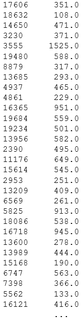
from sklearn.preprocessing import LabelEncoder

encoder = LabelEncoder()
housing_cat = housing["ocean_proximity"]
housing_cat_encoded = encoder.fit_transform(housing_cat)
housing_cat_encoded
OneHotEncoder
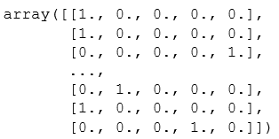
The principle is to create a binary attribute, which is 1 (otherwise 0) when the classification is <1H OCEAN, 1 (otherwise 0) when the classification is INLAND, and 1 (otherwise 0), and so on.This is called One-Hot Encoding because only one attribute equals 1 (hot) and the rest is 0 (cold).
Note: fit_transform() is used for a 2D array, and housing_cat_encoded` is a 1D array, so you need to deform it
from sklearn.preprocessing import OneHotEncoder

encoder = OneHotEncoder()
housing_cat_1hot = encoder.fit_transform(housing_cat_encoded.reshape(-1,1))
# housing_cat_1hot The result is a sparse matrix, where only nonzero items are stored.This is to save memory when there are many classifications.Convert it to numpy Arrays need to be used toarray function
housing_cat_1hot.toarray()
LabelBinarizer
Using the LabelBinarizer class, we can perform these two transformations in one step (from text classification to integer classification, and from integer classification to heat vector)