The goal of regression problem prediction is continuous variable

data description

# Import Boston house price data reader from sklearn.datasets
from sklearn.datasets import load_boston

# Read the house price data from and store it in the variable boston
boston = load_boston

# Output data description
boston.DESCR

Number of Instances: 506
Number of Attributes: 13 numeric/categorical predictive.Median Value (attribute 14) is usually the target.
Missing Attribute Values: None
It can be seen from the above that there are 506 data of housing prices in Boston area, each of which includes 13 numerical characteristic descriptions and target housing prices (average). In addition, there are no missing attribute / characteristic values in the data

data processing

from sklearn.model_selection import train_test_split
import numpy as np

X = boston.data
y = boston.target

# Randomly sampling 25% of the data to build test samples, the rest as training samples
X_train, X_test, y_train, y_test = train_test_split(X, y, test_size=0.25, random_state=33)

# Analyze the difference of regression target value
print("The max target value is", np.max(boston.target))
print("The min target value is", np.min(boston.target))
print("The average target value is", np.mean(boston.target))

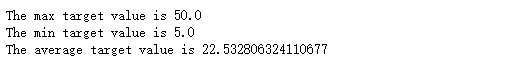
In the above data exploration, we can find that there is a large difference between the predicted target house prices, so we need to standardize the characteristics and target values

# Import data standardization module from sklearn.preprocessing
from sklearn.preprocessing import StandardScaler

# Initialize the standardizer for feature and target values respectively
ss_X = StandardScaler()
ss_y = StandardScaler()

# Standardize the characteristics and target values of training and test data respectively
X_train = ss_X.fit_transform(X_train)
X_test = ss_X.transform(X_test)
y_train = ss_y.fit_transform(y_train.reshape(-1,1))
y_test = ss_y.transform(y_test.reshape(-1,1))

Standardized training target set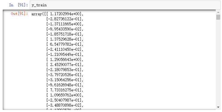

Standardized verification target set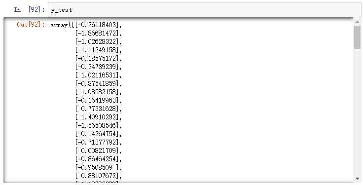

Try a linear model

Here we try to use the linear regression model LinearRegression and sgdregger

# Import LinearRegression from sklearn.linear? Model
from sklearn.linear_model import LinearRegression

# Initializing the linear regression with the default configuration
lr = LinearRegression()

# Parameter estimation using training data
lr.fit(X_train, y_train)

# Regression prediction of test data
lr_y_predict = lr.predict(X_test)

# Import sgdregger from sklearn.linear'u model
from sklearn.linear_model import SGDRegressor

# Initializing the linear regression sgdregger with the default configuration
sgdr = SGDRegressor()

# Parameter estimation using training data
sgdr.fit(X_train, y_train)

# Regression prediction of test data
sgdr_y_predict = sgdr.predict(X_test)

Linear model evaluation

By mean absolute error, mean square error, R-squared evaluation model
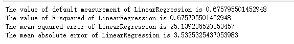
Evaluation of LinearRegression

# Use the evaluation module of LinearRegression model to output the evaluation results
print('The value of default measurement of LinearRegression is', lr.score(X_test, y_test))

# From sklearn.metrics, import R2 ﹐ score, mean ﹐ squared ﹐ error and mean ﹐ absolute ﹐ error for regression performance evaluation
from sklearn.metrics import r2_score, mean_squared_error, mean_absolute_error

# Use R2? Score module and output the evaluation results
print('The value of R-squared of LinearRegression is', r2_score(y_test, lr_y_predict))

# Use the mean squared error module and output the evaluation results
print('The mean squared error of LinearRegression is', mean_squared_error(ss_y.inverse_transform(y_test), ss_y.inverse_transform(lr_y_predict)))

# Use the mean absolute error module and output the evaluation results
print('The mean absolute error of LinearRegression is', mean_absolute_error(ss_y.inverse_transform(y_test), ss_y.inverse_transform(lr_y_predict)))

Sgdregger evaluation

# Use the evaluation module of sgdregger model to output the evaluation results
print('The value of default measurement of SGDRegression is', sgdr.score(X_test, y_test))

# From sklearn.metrics, import R2 ﹐ score, mean ﹐ squared ﹐ error and mean ﹐ absolute ﹐ error for regression performance evaluation
from sklearn.metrics import r2_score, mean_squared_error, mean_absolute_error

# Use the R2? Score module and output the evaluation results
print('The value of R-squared of SGDRegressor is', r2_score(y_test, sgdr_y_predict))

# Use the mean squared error module and output the evaluation results
print('The mean squared error of SGDRegressor is', mean_squared_error(ss_y.inverse_transform(y_test), ss_y.inverse_transform(sgdr_y_predict)))

# Use the mean absolute error module and output the evaluation results
print('The mean absolute error of SGDRegressor is', mean_absolute_error(ss_y.inverse_transform(y_test), ss_y.inverse_transform(sgdr_y_predict)))

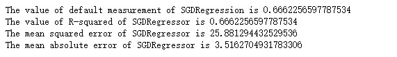
It can be seen that the scoring function of the model is the R-squared index
Sgdregger can save a lot of computing time without losing too much performance when it faces the task of huge training data scale. According to the suggestions of scikit learn website, if the data scale is more than 100000, it is recommended to use the random gradient method to estimate the parameter model

Try support vector machine model

Continue to use the segmented and processed training data and test data
Try three kinds of support vector machine models with different kernel functions

# Importing support vector machine (regression) model from sklearn.svm
from sklearn.svm import SVR

# Support vector machine with linear kernel function is used for regression training, and test samples are predicted
linear_svr = SVR(kernel='linear')
linear_svr.fit(X_train, y_train)
linear_svr_y_predict = linear_svr.predict(X_test)

# Support vector machine with polynomial kernel function is used for regression training, and test samples are predicted
poly_svr = SVR(kernel='poly')
poly_svr.fit(X_train, y_train)
poly_svr_y_predict = poly_svr.predict(X_test)

# Support vector machine with radial vector kernel function is used for regression training, and test samples are predicted
rbf_svr = SVR(kernel='rbf')
rbf_svr.fit(X_train, y_train)
rbf_svr_y_predict = rbf_svr.predict(X_test)

Model assessment

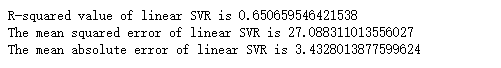
Linear kernel support vector machine

# Import R-squared, MSE and MAE from sklearn.metrics for regression performance evaluation
from sklearn.metrics import r2_score, mean_squared_error, mean_absolute_error

# Output evaluation results
print('R-squared value of linear SVR is', linear_svr.score(X_test, y_test))

# Use the mean squared error module and output the evaluation results
print('The mean squared error of linear SVR is', mean_squared_error(ss_y.inverse_transform(y_test), ss_y.inverse_transform(linear_svr_y_predict)))

# Use the mean absolute error module and output the evaluation results
print('The mean absolute error of linear SVR is', mean_absolute_error(ss_y.inverse_transform(y_test), ss_y.inverse_transform(linear_svr_y_predict)))

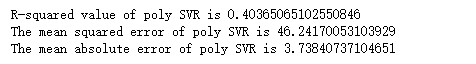
Polynomial kernel support vector machine

# Output evaluation results
print('R-squared value of poly SVR is', poly_svr.score(X_test, y_test))

# Use the mean squared error module and output the evaluation results
print('The mean squared error of poly SVR is', mean_squared_error(ss_y.inverse_transform(y_test), ss_y.inverse_transform(poly_svr_y_predict)))

# Use the mean absolute error module and output the evaluation results
print('The mean absolute error of poly SVR is', mean_absolute_error(ss_y.inverse_transform(y_test), ss_y.inverse_transform(poly_svr_y_predict)))

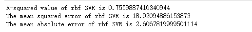
Radial vector kernel function support vector machine

# Output evaluation results
print('R-squared value of rbf SVR is', rbf_svr.score(X_test, y_test))

# Use the mean squared error module and output the evaluation results
print('The mean squared error of rbf SVR is', mean_squared_error(ss_y.inverse_transform(y_test), ss_y.inverse_transform(rbf_svr_y_predict)))

# Use the mean absolute error module and output the evaluation results
print('The mean absolute error of rbf SVR is', mean_absolute_error(ss_y.inverse_transform(y_test), ss_y.inverse_transform(rbf_svr_y_predict)))

Try parameterless model

K-nearest neighbor regression model with two different configurations

# Import KNeighborRegressor from sklearn.neighbors
from sklearn.neighbors import KNeighborsRegressor

# Initialize K-nearest neighbor regression and adjust the configuration so that the prediction method is average regression: weight = uniform '
uni_knr = KNeighborsRegressor(weights='uniform')
uni_knr.fit(X_train, y_train)
uni_knr_y_predict = uni_knr.predict(X_test)

# Initialize the K nearest neighbor regression and adjust the configuration so that the prediction mode is average regression: weight='distance'
dis_knr = KNeighborsRegressor(weights='distance')
dis_knr.fit(X_train, y_train)
dis_knr_y_predict = dis_knr.predict(X_test)

Nonparametric model evaluation

Average regression K-nearest neighbor model

# Using R-squared.MSE and MAE to evaluate the performance of K-nearest neighbor model with average regression configuration on test set
print('R-squared value of uniform-weighted KNeighborRegression:', uni_knr.score(X_test, y_test))
print('The mean squared error of uniform-weighted KNeighborRegression:', mean_squared_error(ss_y.inverse_transform(y_test), ss_y.inverse_transform(uni_knr_y_predict)))
print('The mean absoluate error of uniform-weighted KNeighborRegression:', mean_absolute_error(ss_y.inverse_transform(y_test), ss_y.inverse_transform(uni_knr_y_predict)))

Distance weighted regression K-nearest neighbor model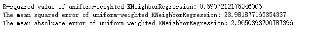

# Using R-squared, MSE and MAE to evaluate the performance of K-nearest-neighbor model configured by distance weighted regression on test set
print('R-squared value of distance-weighted KNeighborRegression:', dis_knr.score(X_test, y_test))
print('The mean squared error of distance-weighted KNeighborRegression:', mean_squared_error(ss_y.inverse_transform(y_test), ss_y.inverse_transform(dis_knr_y_predict)))
print('The mean absoluate error of distance-weighted KNeighborRegression:', mean_absolute_error(ss_y.inverse_transform(y_test), ss_y.inverse_transform(dis_knr_y_predict)))

Try regression tree model

The leaf node of the regression tree returns the mean value of "one mass" training data, rather than specific and continuous prediction values

# Import DecisionTreeRegressor from sklearn.tree
from sklearn.tree import DecisionTreeRegressor

# Initializing DecisionTreeRegressor with default configuration
dtr = DecisionTreeRegressor()

# Building regression tree with Boston house price training data
dtf.fit(X_train, y_train)

# The test data is predicted using a single regression tree configured by default, and the predicted value is stored in the variable DTR ﹣ y ﹣ predict
dtr_y_predict = dtr.predict(X_test)

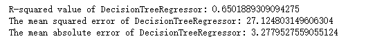
Regression tree model evaluation

# Using R-squared, MSE, and MAE metrics to evaluate the performance of the regression tree of the default configuration on the test set
print('R-squared value of DecisionTreeRegressor:', dtr.score(X_test, y_test))
print('The mean squared error of DecisionTreeRegressor:', mean_squared_error(ss_y.inverse_transform(y_test), ss_y.inverse_transform(dtr_y_predict)))
print('The mean absolute error of DecisionTreeRegressor:', mean_absolute_error(ss_y.inverse_transform(y_test), ss_y.inverse_transform(dtr_y_predict)))

Characteristic analysis

• Tree model can solve the problem of nonlinear characteristics
• The tree model does not require the standardization and unified quantification of features, that is, both numerical and category features can be directly applied to the construction and prediction of tree model
• The tree model can also output the decision-making process intuitively, which makes the prediction result interpretable

At the same time, the tree model has some obvious defects

• Because the tree model can solve the complex nonlinear fitting problem, it is easier to lose the accuracy of new data prediction because the model building is too complex
• The prediction process of tree model from top to bottom will change greatly due to the slight change of data, so the prediction stability is poor
• It is NP hard to build the best tree model based on the training data, that is to say, we can't find the best solution in a limited time, so we can only find some suboptimal solutions with the similar greedy algorithm, which is why we often find higher model performance in multiple suboptimal solutions with the help of integrated model

Try to integrate the model

Extreme random forest, different from the general random forest model, does not randomly select features when constructing a tree's split nodes; instead, it first randomly collects some features, and then uses information entropy and Gini impure to select the best node features
Three models, RandomForestRegressor, ExtraTreesRegressor and gradientboosting regressor, have been tried

# Import RandomForestRegressor, ExtraTreesGressor, and gradientboosting regressor from sklearn.ensemble
from sklearn.ensemble import RandomForestRegressor, ExtraTreesRegressor, GradientBoostingRegressor
# The RandomForestRegressor training model is used to predict the test data, and the results are stored in the variable RFR ﹣ y ﹣ predict
rfr = RandomForestRegressor()
rfr.fit(X_train, y_train)
rfr_y_predict = rfr.predict(X_test)

# The ExtraTreesRegressor training model is used to predict the test data, and the results are stored in the variable ETR ﹤ predict
etr = ExtraTreesRegressor()
etr.fit(X_train, y_train)
etr_y_predict = etr.predict(X_test)

# Use the gradientboosting regression training model, and make a prediction of the test data. The results are stored in the variable GBR ﹣ y ﹣ predict
gbr = GradientBoostingRegressor()
gbr.fit(X_train, y_train)
gbr_y_predict = gbr.predict(X_test)

Integrated model assessment

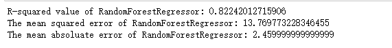
Random regression forest

# Using R-squared.MSE and MAE indicators to evaluate the performance of the random regression forest of the default configuration on the test set
print('R-squared value of RandomForestRegressor:', rfr.score(X_test, y_test))
print('The mean squared error of RandomForestRegressor:', mean_squared_error(ss_y.inverse_transform(y_test), ss_y.inverse_transform(rfr_y_predict)))
print('The mean absoluate error of RandomForestRegressor:', mean_absolute_error(ss_y.inverse_transform(y_test), ss_y.inverse_transform(rfr_y_predict)))

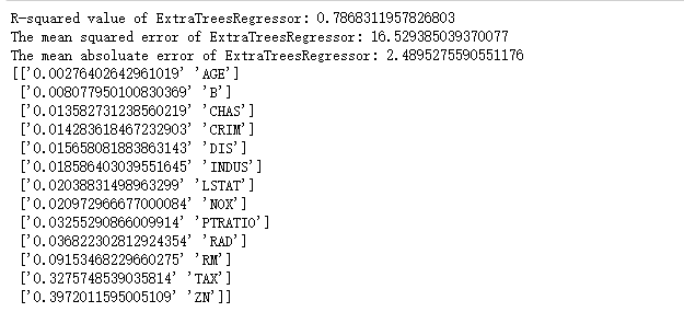
Extreme return to forest

# Using R-squared.MSE and MAE index to evaluate the performance of extreme regression forest on test set
print('R-squared value of ExtraTreesRegressor:', etr.score(X_test, y_test))
print('The mean squared error of ExtraTreesRegressor:', mean_squared_error(ss_y.inverse_transform(y_test), ss_y.inverse_transform(etr_y_predict)))
print('The mean absoluate error of ExtraTreesRegressor:', mean_absolute_error(ss_y.inverse_transform(y_test), ss_y.inverse_transform(etr_y_predict)))

# Using the trained extreme regression forest model, output the contribution of each feature to the prediction target
print(np.sort(list(zip(etr.feature_importances_, boston.feature_names)), axis=0))

Gradient regression forest

# Using R-squared.MSE and MAE index to evaluate the performance of the default forest on the test set
print('R-squared value of GrandientBoostingRegressor:', gbr.score(X_test, y_test))
print('The mean squared error of GrandientBoostingRegressor:', mean_squared_error(ss_y.inverse_transform(y_test), ss_y.inverse_transform(gbr_y_predict)))
print('The mean absoluate error of GrandientBoostingRegressor:', mean_absolute_error(ss_y.inverse_transform(y_test), ss_y.inverse_transform(gbr_y_predict)))

It's not hard to see that integration models often provide better performance and stability