Matlab uses BUGS Markov regime to transform Markov switching random volatility model, sequential Monte Carlo and M-H sampling to analyze time series data

Keywords: Machine Learning AI Deep Learning Data Mining

Original link: http://tecdat.cn/?p=24498

In this example, we consider Markov transformation stochastic volatility model.

statistical model

Give Way Are dependent variables and Unobserved log volatility The stochastic volatility model is defined as follows

Zone variable Following a two-state Markov process with transition probability

Represents the normal distribution of the mean And variance .

BUGS language statistical model

Contents of file "ssv.bug":

file = 'ssv.bug'; % BUGS Model file name

model
{
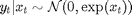
  x\[1\] ~ dnorm(mm\[1\], 1/sig^2)
  y\[1\] ~ dnorm(0, exp(-x\[1\]))

  for (t in 2:tmax)
  {
    c\[t\] ~ dcat(ifelse(c\[t-1\]==1, pi\[1,\], pi\[2,\]))
    mm\[t\] <- alp\[1\] * (c\[t\]==1) + alp\[2\]*(c\[t\]==2) + ph*x\[t-1\]

install

Download the latest version of Matlab
Unzip the archive into a folder
Add program folder to Matlab search path

addpath(path)

General settings

lightblue 
lightred 

% Seed the random number generator for repeatability
if eLan 'matlab', '7.2')
    rnd('state', 0)
else
    rng('default')
end

Load models and data

model parameter

tmax = 100;
sig = .4;

Parse and compile BUGS model and sample data

model(file, data, 'sample', true);
data = model;

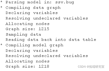
Draw data

figure('nae', 'Lrtrs')
plot(1:tmax, dt.y)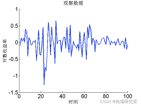

Biips sequence Monte Carlo SMC

Run SMC

n_part = 5000; % Particle number
  {'x'}; % Variables to monitor
 smc =  samples(npart)；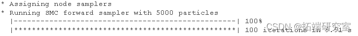

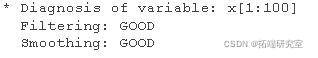
Algorithm diagnosis.

diag   (smc);

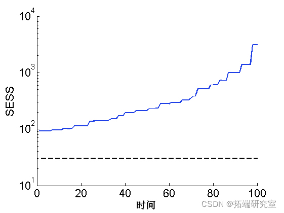
Drawing smoothing ESS

sem(ess)

plot(1:tmax, 30*(tmax,1), '--k')

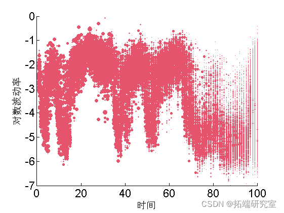
Paint weighted particles

for ttt=1:tttmax
    va = unique(outtt.x.s.vaues(ttt,:));

    wegh = arrayfun(@(x) sum(outtt.x.s.weittt(ttt, outtt.x.s.vaues(ttt,:) == x)), va);

    scatttttter(ttt\*ones(size(va)), va, min(50, .5\*n_parttt*wegh), 'r',...
        'markerf', 'r')
end

Summary statistics

summary(out, 'pro', \[.025, .975\]);

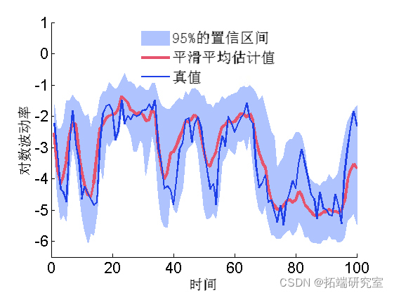
Mapping filter estimation

mean = susmc.x.f.mean;
xfqu = susmc.x.f.quant;
h = fill(\[1:tmax, tmax:-1:1\], \[xfqu{1}; flipud(xfqu{2})\], 0);

plot(1:tmax, mean,)
plot(1:tmax, data.x_true)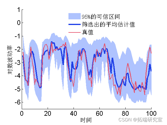

Mapping smoothing estimation

mean = smcx.s.mean;
quant = smcx.s.quant;

plot(1:t_max, mean,  3)
plot(1:t\_max, data.x\_true, 'g')

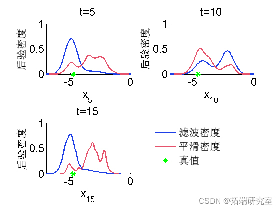
Marginal filtering and smoothing density

kde = density(out);
for k=1:numel(time)
    tk = time(k);
    plot(kde.x.f(tk).x, kde.x.f(tk).f);
    hold on
    plot(kde.x.s(tk).x, kde.x.s(tk).f, 'r');
    plot(data.xtrue(tk));
    box off
end

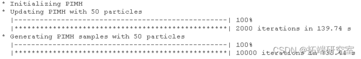
Biips particle independent metropolis Hastings

PIMH parameters

thi= 1;
nprt = 50;

Running PIMH

init(moel, vaibls);
upda(obj, urn, npat); % Pre burn iteration
sample(obj,...
    nier, npat, 'thin', thn);

Some summary statistics

summary(out, 'prs');

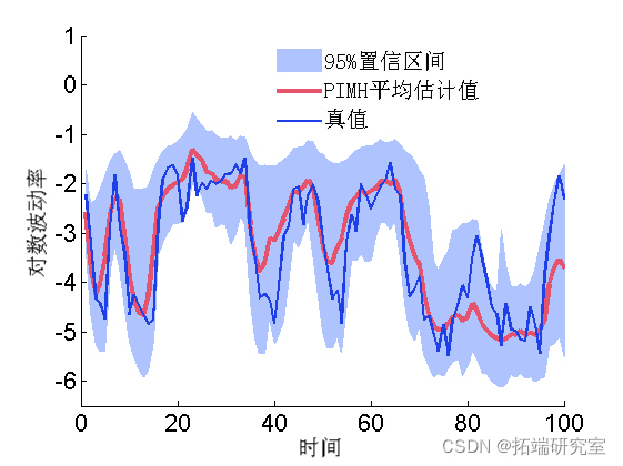
Post mean and quantile

mean = sumx.man;
quant = su.x.qunt;

hold on
plot(1:tax, man, 'r', 'liith', 3)
plot(1:tax, xrue, 'g')

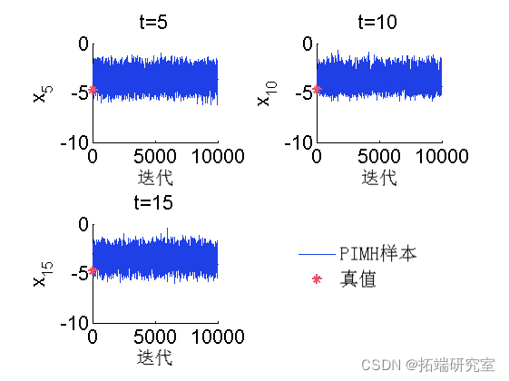
Trace of MCMC samples

for k=1:nmel(timndx)
    tk = tieinx(k);
    sublt(2, 2, k)
    plot(outm.x(tk, :), 'liedh', 1)
    hold on
    plot(0, d_retk), '*g');
    box off
end

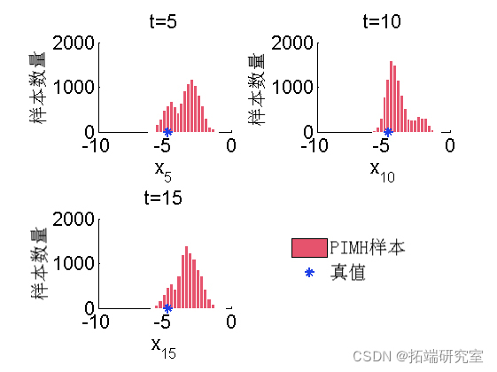
A posteriori histogram

for k=1:numel(tim_ix)
    tk = tim_ix(k);
    subplot(2, 2, k)
    hist(o_hx(tk, :), 20);
    h = fidobj(gca, 'ype, 'ptc');    hold on
    plot(daau(k), 0, '*g');
   
    box off
end

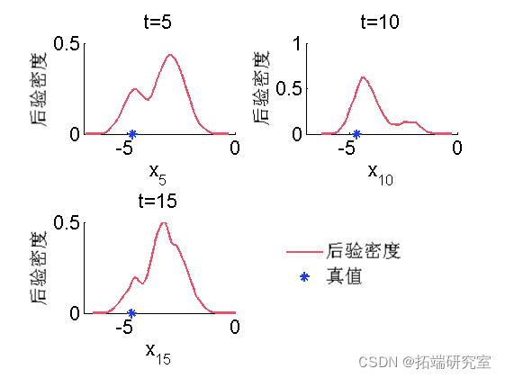
A posteriori kernel density estimation

pmh = desity(otmh);
for k=1:numel(tenx)
    tk = tim_ix(k);
    subplot(2, 2, k)
    plot(x(t).x, dpi.x(tk).f, 'r');
    hold on
    plot(xtrue(tk), 0, '*g');
    box off
end

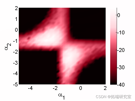
Biips sensitivity analysis

We want to study the sensitivity to parameter values

Algorithm parameters

n= 50; % Particle number
para = {'alpha}; % We want to study the parameters of sensitivity
 % Value grid of two components
pvs = {A(:, B(:';

Run sensitivity analysis using SMC

smcs(modl, par, parvlu, npt);

Plot log marginal likelihood and penalty log marginal likelihood rate

surf(A, B, reshape(ouma_i, sizeA)
box off

Programmer Group