Starting from this article, the author officially began to explain the knowledge related to Python in-depth learning, neural network and artificial intelligence. I hope you like it.
The previous article explained TensorFlow basis and univariate linear prediction cases, as well as Session, variable, incoming value and excitation function; This article will introduce TensorFlow to create regression neural network and Optimizer in detail. This article mainly combines the author's previous blog and the video introduction of "don't bother God". Later, we will explain the specific projects and applications in depth.
Basic articles, I hope to help you. If there are errors or deficiencies in the articles, please Haihan ~ at the same time, I am also a rookie of artificial intelligence. I hope you can grow up with me in this stroke by stroke blog.
Article directory:
- 1, TensorFlow creates a neural layer
- 2, Implementation of recurrent neural network 1. Making virtual data 2. Add neural network layer 3. Calculation error and neural network learning
- 3, Visual analysis of regression neural network
- 4, Optimizer optimizer
- 5, Summary
Code download address:
- https://github.com/eastmountyxz/ AI-for-TensorFlow
- https://github.com/eastmountyxz/ AI-for-Keras
1, TensorFlow creates a neural layer
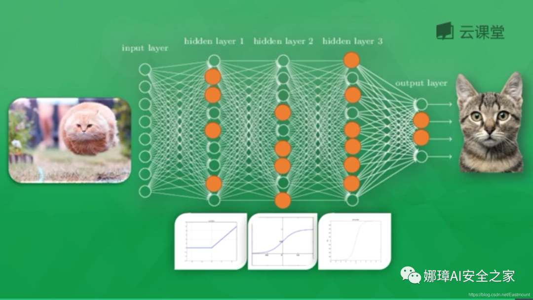
As shown in the figure, the animal cat or dog is identified through the neural network, including Input Layer, Hidden Layer and Output Layer. Each Hidden Layer neuron has an excitation function. The information transmitted by the excited neuron is the most valuable. It also determines the final output result. After massive data training, the final neural network can be used to identify cats or dogs.
In this paper, TensorFlow will continuously train and learn to fit a curve to predict the distribution law of scatter points. First, we need to add a neural Layer and define the Layer as a function to add a neural Layer. The neural Layer is interconnected, from the first input Layer to the hidden Layer, and finally to the output Layer. The function prototype is as follows:
- add_layer(inputs, in_size, out_size, activation_function=None)
- Parameters include input value, number of input nodes, number of output nodes and excitation function (None by default)
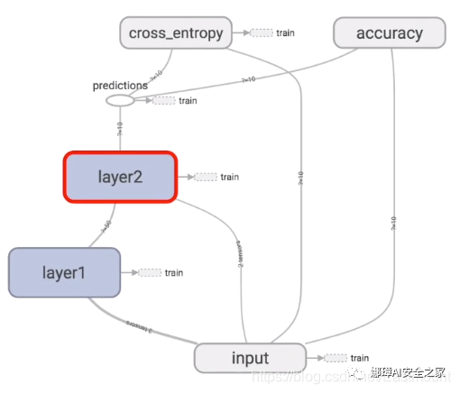
TensorFlow is structured as follows. The input value passes through hidden layers layer1 and layer2, and then there is a prediction value, predictions, cross_entropy is the difference between the calculated value and the real value.
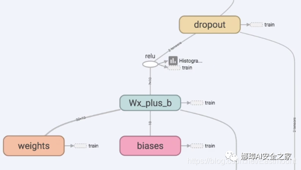
First, the layer we need to make is Layer1 or Layer2. There will be Weights and bias between them. The calculation is located in Wx_ plus_ In B, the excitation function is relu.
Let's start writing the code as follows: (see the notes for details)
# -*- coding: utf-8 -*-
"""
Created on Thu Dec  5 18:52:06 2019
@author: xiuzhang Eastmount CSDN
"""
import tensorflow as tf

#---------------------------------Define neural layer-------------------------------
# Function: input variable input size output size excitation function default None
def add_layer(inputs, in_size, out_size, activation_function=None):
    # The weight is a random variable matrix
    Weights = tf.Variable(tf.random_normal([in_size, out_size]))    #Row * column
    # The initial value of the defined offset is increased by 0.1, which changes in each training
    biases = tf.Variable(tf.zeros([1, out_size]) + 0.1)             #1 row and multiple columns
    # Defines the predicted value of the calculated matrix multiplication
    Wx_plus_b = tf.matmul(inputs, Weights) + biases
    # Activate operation
    if activation_function is None:
        outputs = Wx_plus_b
    else:
        outputs = activation_function(Wx_plus_b)

    return outputs
2, Implementation of recurrent neural network
Next, the first neural network code is implemented, and the steps are as follows:
1. Making virtual data
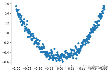
300 random points are generated through numpy.linspace for training to form virtual data of y=x^2-0.5. The code is as follows:
import tensorflow as tf
import numpy as np
#---------------------------------Define neural layer---------------------------------
# Function: input variable input size output size excitation function default None
def add_layer(inputs, in_size, out_size, activation_function=None):
    # The weight is a random variable matrix
    Weights = tf.Variable(tf.random_normal([in_size, out_size]))    #Row * column
    # The initial value of the defined offset is increased by 0.1, which changes in each training
    biases = tf.Variable(tf.zeros([1, out_size]) + 0.1)             #1 row and multiple columns
    # Defines the predicted value of the calculated matrix multiplication
    Wx_plus_b = tf.matmul(inputs, Weights) + biases
    # Activate operation
    if activation_function is None:
        outputs = Wx_plus_b
    else:
        outputs = activation_function(Wx_plus_b)

    return outputs

#---------------------------------Construction data---------------------------------
# input
x_data = np.linspace(-1, 1, 300)[:,np.newaxis]   #dimension
# Noise
noise = np.random.normal(0, 0.05, x_data.shape)  #Mean value 0, variance 0.05
# output
y_data = np.square(x_data) -0.5 + noise

# Set the passed in values xs and ys
xs = tf.placeholder(tf.float32, [None, 1]) #x_data passed in to xs
ys = tf.placeholder(tf.float32,[None, 1]) #y_data passed in to ys

#---------------------------------Visual analysis---------------------------------
import matplotlib.pyplot as plt

# Define picture box
fig = plt.figure()
ax = fig.add_subplot(1,1,1)
# Scatter diagram
ax.scatter(x_data, y_data)
plt.show()
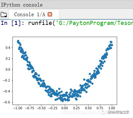
Here, the scatter diagram is simply drawn through matplotlib, and the output result is shown in the figure below, which basically meets the following requirements: y_data = np.square(x_data) -0.5 + noise.
2. Add neural network layer
The hidden layer L1 and the output layer prediction are defined.
- L1 = add_layer(xs, 1, 10, activation_function=tf.nn.relu) The input is xs, 1-dimensional data, 10 neurons, relu nonlinear excitation function
- prediction = add_layer(L1, 10, 1, activation_function=None) Input is L1 output value, in_ For neuron 10 with size L1, L2 output is assumed to be the final output
The complete code is shown in the figure below:
# -*- coding: utf-8 -*-
"""
Created on Thu Dec  5 18:52:06 2019
@author: xiuzhang Eastmount CSDN
"""
import tensorflow as tf
import numpy as np

#---------------------------------Define neural layer---------------------------------
# Function: input variable input size output size excitation function default None
def add_layer(inputs, in_size, out_size, activation_function=None):
    # The weight is a random variable matrix
    Weights = tf.Variable(tf.random_normal([in_size, out_size]))    #Row * column
    # The initial value of the defined offset is increased by 0.1, which changes in each training
    biases = tf.Variable(tf.zeros([1, out_size]) + 0.1)             #1 row and multiple columns
    # Defines the predicted value of the calculated matrix multiplication
    Wx_plus_b = tf.matmul(inputs, Weights) + biases
    # Activate operation
    if activation_function is None:
        outputs = Wx_plus_b
    else:
        outputs = activation_function(Wx_plus_b)

    return outputs

#---------------------------------Construction data---------------------------------
# input
x_data = np.linspace(-1, 1, 300)[:,np.newaxis]   #dimension
# Noise
noise = np.random.normal(0, 0.05, x_data.shape)  #Mean value 0, variance 0.05
# output
y_data =np.square(x_data) -0.5 + noise

# Set the passed in values xs and ys
xs = tf.placeholder(tf.float32, [None, 1]) #x_data passed in to xs
ys = tf.placeholder(tf.float32,[None, 1]) #y_data passed in to ys

#---------------------------------Visual analysis---------------------------------
import matplotlib.pyplot as plt

# Define picture box
fig = plt.figure()
ax = fig.add_subplot(1,1,1)
# Scatter diagram
ax.scatter(x_data, y_data)
# Continuous display
plt.ion()
plt.show()

#---------------------------------Defining neural networks---------------------------------
# One input layer: x_data has only one attribute, so it has only one neuron
# One output layer: y_data has only one attribute, so it has only one neuron
# One hidden layer: 10 neurons

# Hidden layer
L1 = add_layer(xs, 1, 10, activation_function=tf.nn.relu)

# Output layer
prediction = add_layer(L1, 10, 1, activation_function=None)
3. Calculation error and neural network learning
Define the calculation error of loss variable, that is, the difference between the predicted value and the real value; Then define the gradient descent optimizer to make the predicted value closer to the real value through gradient descent. Finally, initialize and calculate the error in the Session, and output the operation result every 50 steps.
# -*- coding: utf-8 -*-
"""
Created on Thu Dec  5 18:52:06 2019
@author: xiuzhang Eastmount CSDN
"""
import tensorflow as tf
import numpy as np

#---------------------------------Define neural layer---------------------------------
# Function: input variable input size output size excitation function default None
def add_layer(inputs, in_size, out_size, activation_function=None):
    # The weight is a random variable matrix
    Weights = tf.Variable(tf.random_normal([in_size, out_size]))    #Row * column
    # The initial value of the defined offset is increased by 0.1, which changes in each training
    biases = tf.Variable(tf.zeros([1, out_size]) + 0.1)             #1 row and multiple columns
    # Defines the predicted value of the calculated matrix multiplication
    Wx_plus_b = tf.matmul(inputs, Weights) + biases
    # Activate operation
    if activation_function is None:
        outputs = Wx_plus_b
    else:
        outputs = activation_function(Wx_plus_b)

    return outputs

#---------------------------------Construction data---------------------------------
# input
x_data = np.linspace(-1, 1, 300)[:,np.newaxis]   #dimension
# Noise
noise = np.random.normal(0, 0.05, x_data.shape)  #Mean value 0, variance 0.05
# output
y_data =np.square(x_data) -0.5 + noise

# Set the passed in values xs and ys
xs = tf.placeholder(tf.float32, [None, 1]) #x_data passed in to xs
ys = tf.placeholder(tf.float32,[None, 1]) #y_data passed in to ys

#---------------------------------Visual analysis---------------------------------
import matplotlib.pyplot as plt

# Define picture box
fig = plt.figure()
ax = fig.add_subplot(1,1,1)
# Scatter diagram
ax.scatter(x_data, y_data)
# Continuous display
plt.ion()
plt.show()

#---------------------------------Defining neural networks---------------------------------
# One input layer: x_data has only one attribute, so it has only one neuron
# One output layer: y_data has only one attribute, so it has only one neuron
# One hidden layer: 10 neurons

# Hidden layer
L1 = add_layer(xs, 1, 10, activation_function=tf.nn.relu)

# Output layer
prediction = add_layer(L1, 10, 1, activation_function=None)

#------------------------------Define loss and initialization-------------------------------
# Average error between predicted value and real value - > sum - > square (real value - predicted value)
loss = tf.reduce_mean(tf.reduce_sum(tf.square(ys - prediction),
                     reduction_indices=[1]))

# The training efficiency is usually less than 1, which can be set to 0.1 for comparison
train_step = tf.train.GradientDescentOptimizer(0.1).minimize(loss) #Reduce error

# initialization
init = tf.initialize_all_variables()

# function
sess = tf.Session()
sess.run(init)

#---------------------------------Neural network learning---------------------------------

# Learn 1000 times
n = 1
for i in range(1000):
    # train
    sess.run(train_step, feed_dict={xs:x_data, ys:y_data}) #Assume all data x_data
    # As long as the output result passes through place_ To run holder, you need to pass in parameters
    if i % 50==0:
        print(sess.run(loss, feed_dict={xs:x_data, ys:y_data}))
The output results are shown in the figure below. The output results are output every 50 steps. The error of the first time is 0.45145842 and the error of the second time is 0.012015346. The error is decreasing, indicating that the neural network is improving the accuracy of prediction or learning something.
0.45145842
0.012015346
0.008982641
0.008721641
0.0085632615
0.008296631
0.0078961495
0.0074299597
0.0069189137
0.0063963127
0.0058622854
0.00548969
0.0051686876
0.0048802416
0.0046461136
0.0044451333
0.0042808857
0.004134449
0.0040101893
0.0039141406
Here, the definition and operation process of the whole neural network are described, including the definition of neural layer, error setting, initialization and operation, and then the visual analysis is started.
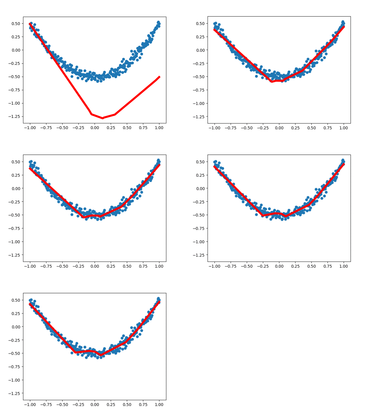
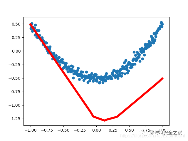
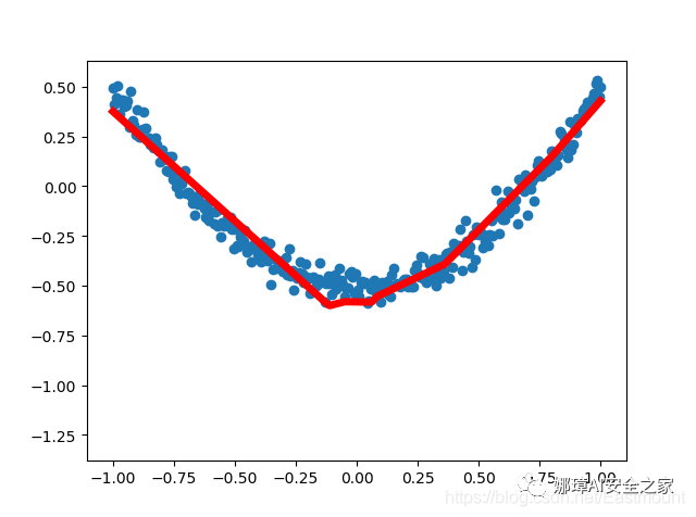
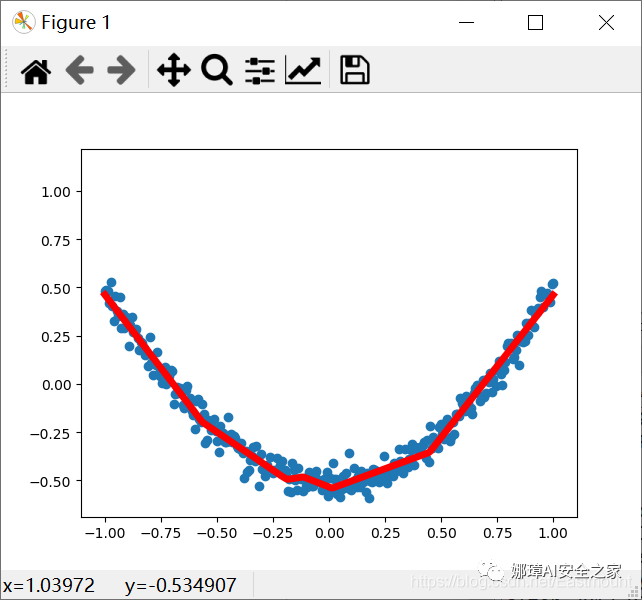
3, Visual analysis of regression neural networkIn order to more intuitively understand how the neural network optimizes the results, we use matplotlib for visual analysis. From the earliest unreasonable figure to the following basic fitting, the loss error is decreasing, indicating that the real value and predicted value of the neural network are constantly updated and close, and the neural network operates normally.
First run result:
Results of the fourth operation:
Results of the 20th operation:
The complete code and comments are as follows:
# -*- coding: utf-8 -*-
"""
Created on Thu Dec  5 18:52:06 2019
@author: xiuzhang Eastmount CSDN
"""
import tensorflow as tf
import numpy as np

#---------------------------------Define neural layer---------------------------------
# Function: input variable input size output size excitation function default None
def add_layer(inputs, in_size, out_size, activation_function=None):
    # The weight is a random variable matrix
    Weights = tf.Variable(tf.random_normal([in_size, out_size]))    #Row * column
    # The initial value of the defined offset is increased by 0.1, which changes in each training
    biases = tf.Variable(tf.zeros([1, out_size]) + 0.1)             #1 row and multiple columns
    # Defines the predicted value of the calculated matrix multiplication
    Wx_plus_b = tf.matmul(inputs, Weights) + biases
    # Activate operation
    if activation_function is None:
        outputs = Wx_plus_b
    else:
        outputs = activation_function(Wx_plus_b)

    return outputs

#---------------------------------Construction data---------------------------------
# input
x_data = np.linspace(-1, 1, 300)[:,np.newaxis]   #dimension
# Noise
noise = np.random.normal(0, 0.05, x_data.shape)  #Mean value 0, variance 0.05
# output
y_data =np.square(x_data) -0.5 + noise

# Set the passed in values xs and ys
xs = tf.placeholder(tf.float32, [None, 1]) #x_data passed in to xs
ys = tf.placeholder(tf.float32,[None, 1]) #y_data passed in to ys

#---------------------------------Visual analysis---------------------------------
import matplotlib.pyplot as plt

# Define picture box
fig = plt.figure()
ax = fig.add_subplot(1,1,1)
# Scatter diagram
ax.scatter(x_data, y_data)
# Continuous display
plt.ion()
plt.show()

#---------------------------------Defining neural networks---------------------------------
# Hidden layer
L1 = add_layer(xs, 1, 10, activation_function=tf.nn.relu)

# Output layer
prediction = add_layer(L1, 10, 1, activation_function=None)

#------------------------------Define loss and initialization-------------------------------

# Average error between predicted value and real value - > sum - > square (real value - predicted value)
loss = tf.reduce_mean(tf.reduce_sum(tf.square(ys - prediction),
                     reduction_indices=[1]))

# The training efficiency is usually less than 1, which can be set to 0.1 for comparison
train_step = tf.train.GradientDescentOptimizer(0.1).minimize(loss) #Reduce error

# initialization
init = tf.initialize_all_variables()

# function
sess = tf.Session()
sess.run(init)

#---------------------------------Neural network learning---------------------------------

# Learn 1000 times
n = 1
for i in range(1000):
    # train
    sess.run(train_step, feed_dict={xs:x_data, ys:y_data}) #Assume all data x_data
    # As long as the output result passes through place_ To run holder, you need to pass in parameters
    if i % 50==0:
        #print(sess.run(loss, feed_dict={xs:x_data, ys:y_data}))

        try:
            # Ignore the first error and subsequently remove the first line segment of lines
            ax.lines.remove(lines[0])
        except Exception:
            pass

        # forecast
        prediction_value = sess.run(prediction, feed_dict={xs:x_data})
        # Set the line width to 5 red
        lines = ax.plot(x_data, prediction_value, 'r-', lw=5)
        # suspend
        plt.pause(0.1)
        # Save picture
        name = "test" + str(n) + ".png"
        plt.savefig(name)
        n =  n + 1
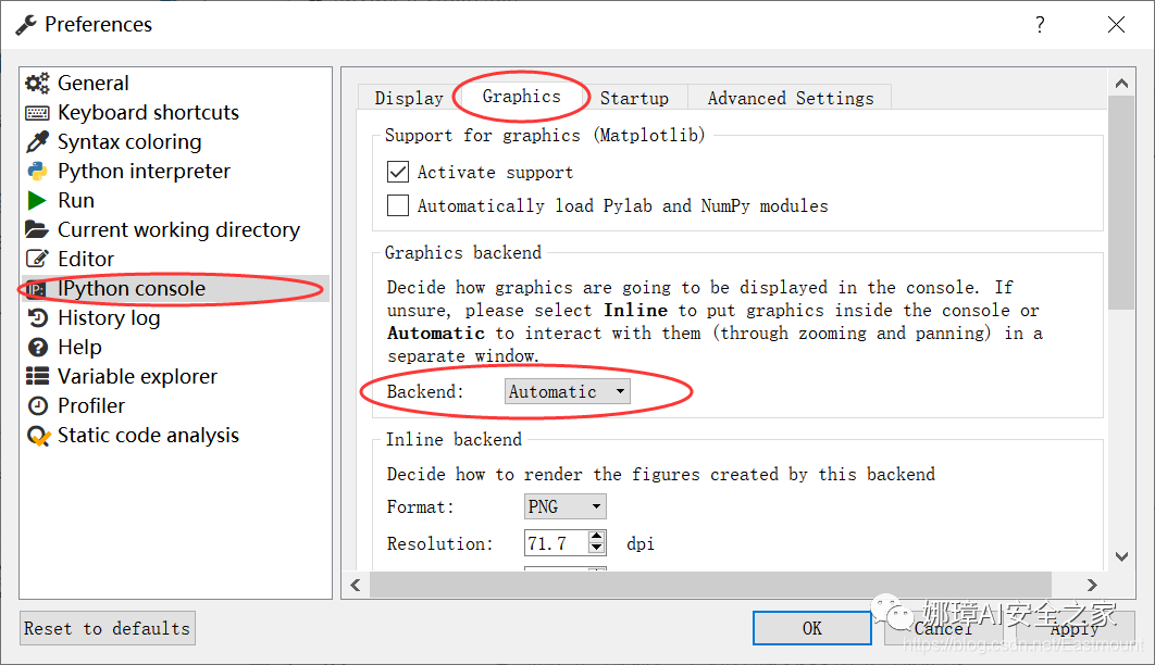
Note: in Spyder software running code, figure is generally displayed in IPython console, as shown in the following figure. The figure is relatively small and cannot be operated. At the same time, dynamic figure cannot be displayed in IPython console. You need to set a separate pop-up window to solve this problem.
The steps to set a separate pop-up window in Spyder software are: Tools – > preferences – > IPython console – > graphics – > graphics backend – > backend – > set to Automatic, as shown in the figure below.
If it is set to Inline, figure is displayed in the IPython console. Finally, the Spyder software needs to be restarted. If it is not restarted, the setting effect cannot be realized. In this way, a separate window can be displayed, and the dynamic figure display can be realized, such as the curve dynamic fitting effect shown in the figure.
Reference: figure is displayed in a separate pop-up window in Spyder and the setting of dynamic figure display is solved
4, Optimizer optimizer
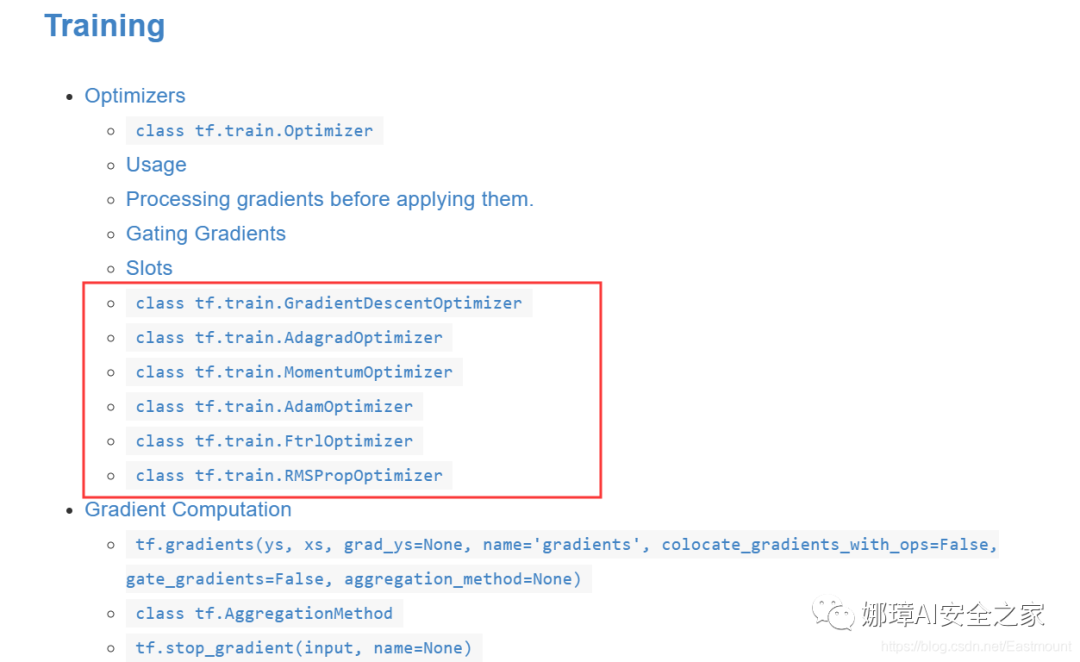
class tf.train.Optimizer is the base class of the optimizers class. This class defines the API for adding an operation when training the model. Basically, you won't use this class directly, but you will use its subclasses, such as GradientDescentOptimizer, AdagradOptimizer, MomentumOptimizer, etc.
There are many different kinds of optimizers. The most basic one is gradientsdesentoptimizer, which is also the most important or basic linear optimization in machine learning. The common optimizers officially given are shown in the figure below:
Official website:
- http://www.tensorfly.cn/tfdoc/ api_docs/python/train.html
- https://tensorflow.google.cn/versions/ r1.15/api_docs/python/tf/train/Optimizer
It introduces seven common optimizers, including:
- class tf.train.GradientDescentOptimizer
- class tf.train.AdagradOptimizer
- class tf.train.AdadeltaOptimizer
- class tf.train.MomentumOptimizer
- class tf.train.AdamOptimizer
- class tf.train.FtrlOptimizer
- class tf.train.RMSPropOptimizer
Let's share the usage of optimizer with readers in combination with the teacher's course of "don't bother".
- GradientDescentOptimizer (gradient descent) depends on the size of the incoming data. For example, if only one tenth of the total data is transmitted, the gradientdescent optimizer becomes STD. it only considers part of the data and learns part by part. Its advantage is that it can learn the path to the Global minimum faster.
- MomentumOptimizer It is based on the change of learning efficiency. It not only considers the learning efficiency of this step, but also loads the learning efficiency trend of the previous step, and then adds the learning of this step to the previous step_ Rate, which will reach the global minimum faster than the Gradient Descent Optimizer.
- RMSPropOptimizer Google uses it to optimize the learning efficiency of alpha dogs.
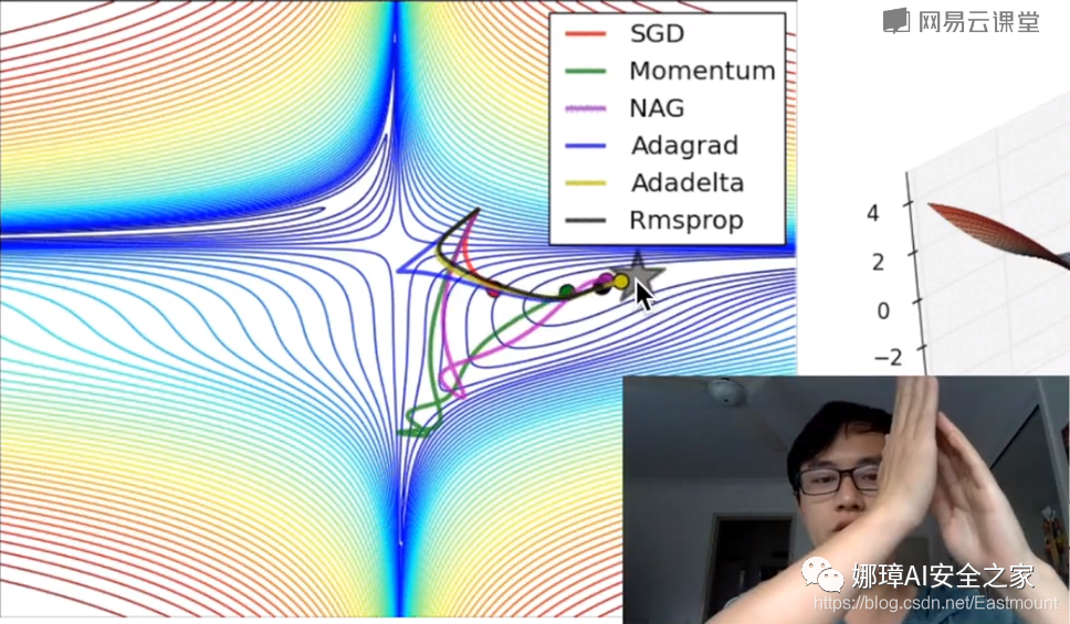
The following figure compares and analyzes various optimizers through visualization. There are different learning paths in the process of machine learning from target learning to optimization. Since Momentum considers the learning_rate in the previous step, the path will be very long; GradientDescent's learning time will be very slow.
- If you are a beginner, it is recommended to use GradientDescentOptimizer;
- If you have a certain foundation, you can consider two commonly used optimizers, momentum optimizer and Adam optimizer;
- At a higher level, you can try to learn the RMSPropOptimizer optimizer.
In short, you'd better select the appropriate optimizer according to the specific research problems.
5, Summary
I'm really busy writing this article late at night. I hope this basic article will help you. If there are errors or deficiencies in the article, please forgive me~
References, thank you for your articles and videos. I recommend you to follow Mr. Mo fan. He is my introductory teacher of artificial intelligence.
- [1] Introduction to neural networks and machine learning - author's article
- [2] Stanford machine learning video Professor NG: https://class.coursera.org/ml/class/index
- [3] Book "artificial intelligence in game development"
- [4] Netease cloud don't bother teacher video (strong push): https://study.163.com/course/courseLearn.htm?courseId=1003209007
- [5] Neural network excitation function - deep learning
- [6] tensorflow Architecture - NoMorningstar
- [7] Tensorflow 2.0 introduction to low level api - GumKey
- [8] Fundamentals of tensorflow - kk123k
- [9] Tensorflow basic knowledge sorting - sinat_ thirty-six million one hundred and ninety thousand six hundred and forty-nine
- [10] Deep learning (II): TensorFlow Basics - the sea of hichri
- [11] tensorflow basic concept - lusic01
- [12] tensorflow: activation function - haoji007
- [13] AI = > tensorflow 2.0 syntax - tensor & basic function (I)