This series of articles is to explain Python OpenCV image processing knowledge. In the early stage, it mainly explains the introduction of image and the basic usage of OpenCV. In the middle stage, it explains various algorithms of image processing, including image sharpening operator, image enhancement technology, image segmentation, etc. in the later stage, it studies image recognition and image classification application in combination with in-depth learning. I hope the article is helpful to you. If there are deficiencies, please forgive me~
All source code of this series in github:
- https://github.com/eastmountyxz/ ImageProcessing-Python
The previous article introduced the basic knowledge of OpenCV and Numpy image processing, including reading and modifying pixels, and geometric drawing. This article mainly explains how Python calls OpenCV to obtain image attributes, intercept ROI regions of interest, and process image channels. The knowledge points are as follows:
- 1, Get image properties
- 2, Get ROI region of interest
- 3, Image channel processing
- 4, Image type conversion
1, Get image properties
The most common attributes of an image include three: image shape, pixel size, and image type.
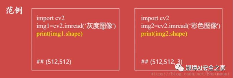
1. Shape shape Get the shape of the image through the shape keyword, and return the primitive including the number of rows, columns and channels. The gray image returns the number of rows and columns, and the color image returns the number of rows, columns and channels. As shown in the figure below:
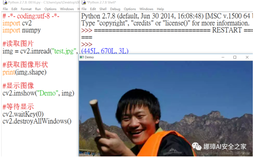
# -*- coding:utf-8 -*-
import cv2
import numpy

#Read picture
img = cv2.imread("yxz.png", cv2.IMREAD_UNCHANGED)

#Get image shape
print(img.shape)

#Display image
cv2.imshow("Demo", img)

#Wait for display
cv2.waitKey(0)
cv2.destroyAllWindows()
The output results are shown in the following figure: (445L, 670L, 3L). The figure has 445 rows, 670 columns, pixels and 3 channels.
2. Number of pixels - size Obtain the number of pixels of the image through the size keyword, where the gray image returns the number of rows * the number of columns, and the color image returns the number of rows * the number of columns * the number of channels. The code is as follows:
# -*- coding:utf-8 -*-
import cv2
import numpy

#Read picture
img = cv2.imread("yxz.png", cv2.IMREAD_UNCHANGED)

#Get image shape
print(img.shape)

#Gets the number of pixels
print(img.size)
Output results:
- (445L, 670L, 3L)
- 894450
3. Image type dtype
Get the data type of the image through the dtype keyword, usually return uint8. The code is as follows:
# -*- coding:utf-8 -*-
import cv2
import numpy

#Read picture
img = cv2.imread("yxz.png", cv2.IMREAD_UNCHANGED)

#Get image shape
print(img.shape)

#Gets the number of pixels
print(img.size)

#Get image type
print(img.dtype)
Output results:
- (445L, 670L, 3L)
- 894450
- uint8
2, Get ROI region of interest
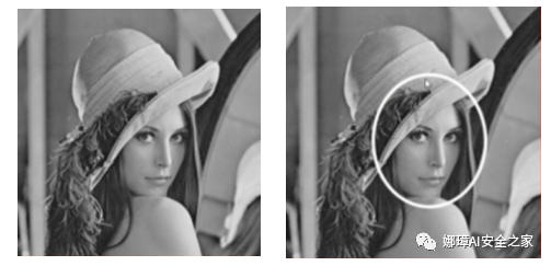
ROI (Region of Interest) refers to the Region of Interest that needs to be processed from the processed image in the form of box, circle, ellipse, irregular polygon, etc. ROI regions of interest can be obtained by various operators and functions, which are widely used in hot spot map, face recognition, image segmentation and other fields. Obtain the face contour of Lena diagram as shown in the figure.
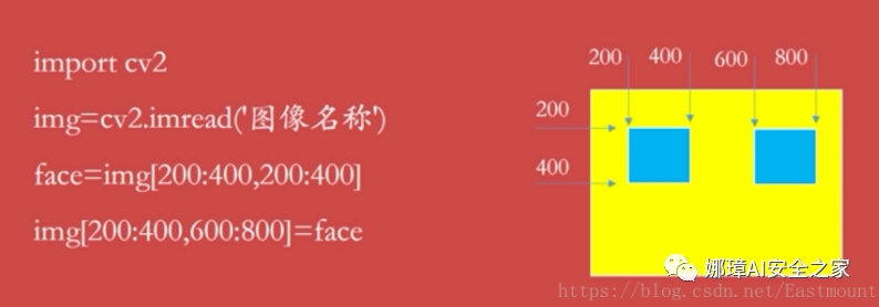
ROI regions can be obtained directly through the pixel matrix, such as img[200:400, 200:400].
The code is as follows:
# -*- coding:utf-8 -*-
import cv2
import numpy as np
#Read picture
img = cv2.imread("test.jpg", cv2.IMREAD_UNCHANGED)
#Define BGR corresponding to 200 * 100 matrix 3
face = np.ones((200, 100, 3))
#Display original image
cv2.imshow("Demo", img)
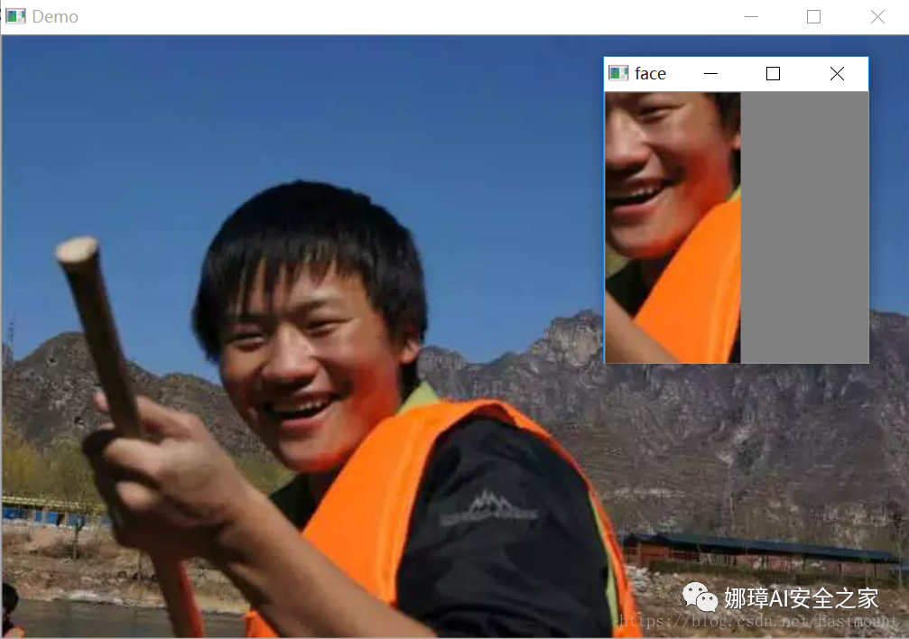
#Show ROI area
face = img[200:400, 200:300]
cv2.imshow("face", face)
#Wait for display
cv2.waitKey(0)
cv2.destroyAllWindows()
The output results are shown in the figure below:
The following is a fusion experiment of the extracted ROI image. The code is as follows:
# -*- coding:utf-8 -*-
import cv2
import numpy as np
#Read picture
img = cv2.imread("test.jpg", cv2.IMREAD_UNCHANGED)
#Define BGR corresponding to 300 * 100 matrix 3
face = np.ones((200, 200, 3))
#Display original image
cv2.imshow("Demo", img)
#Show ROI area
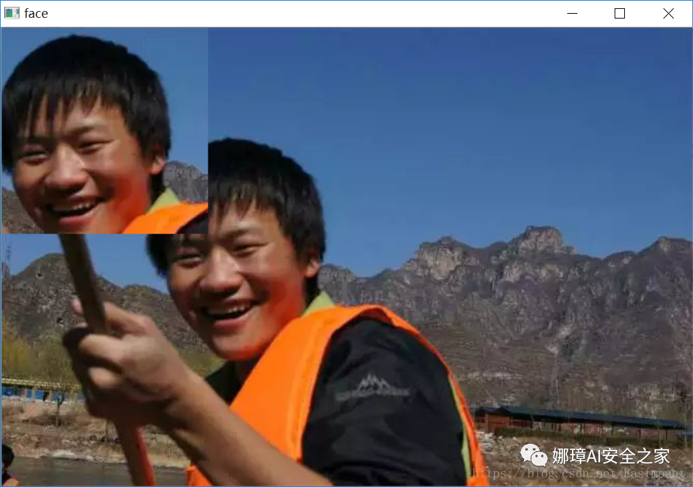
face = img[100:300, 150:350]
img[0:200,0:200] = face
cv2.imshow("face", img)
#Wait for display
cv2.waitKey(0)
cv2.destroyAllWindows()
Fuse the extracted head to the upper left corner of the image, as shown in the following figure:
If you want to fuse two images, you only need to read another image, and the method principle is similar. The code is as follows:
# -*- coding:utf-8 -*-
import cv2
import numpy as np
#Read picture
img = cv2.imread("yxz.jpg", cv2.IMREAD_UNCHANGED)
test = cv2.imread("na.jpg", cv2.IMREAD_UNCHANGED)
#Define BGR corresponding to 300 * 100 matrix 3
face = np.ones((200, 200, 3))
#Display original image
cv2.imshow("Demo", img)
#Show ROI area
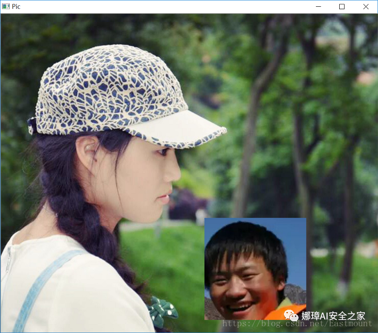
face = img[100:300, 150:350]
test[400:600,400:600] = face
cv2.imshow("Pic", test)
#Wait for display
cv2.waitKey(0)
cv2.destroyAllWindows()
The output results are shown in the figure below:
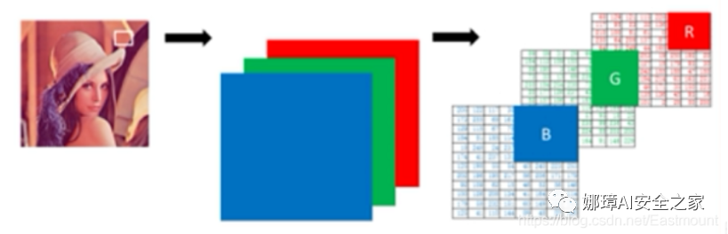
3, Image channel processing
OpenCV implements the processing of image channels through split() function and merge() function, including channel separation and channel merging.
1. Channel split The color image read by OpenCV is composed of three primary colors: B, G and R. different channels can be obtained through the following code.
- b = img[:, :, 0]
- g = img[:, :, 1]
- r = img[:, :, 2]
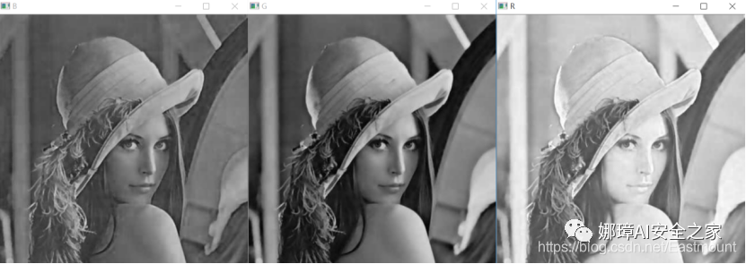
You can also use the split() function to split channels. The following is the code to split different channels and then display them.
- mv = split(m[, mv]) – m represents the input multichannel array – mv represents the output array or vector container
# -*- coding:utf-8 -*-
import cv2
import numpy as np

#Read picture
img = cv2.imread("Lena.png")

#Split channel
b, g, r = cv2.split(img)

#Display original image
cv2.imshow("B", b)
cv2.imshow("G", g)
cv2.imshow("R", r)

#Wait for display
cv2.waitKey(0)
cv2.destroyAllWindows()
The display result is shown in the figure, which shows the color components of B, G and R channels.
You can also obtain different channel colors. The core code is:
- b = cv2.split(a)[0]
- g = cv2.split(a)[1]
- r = cv2.split(a)[2]
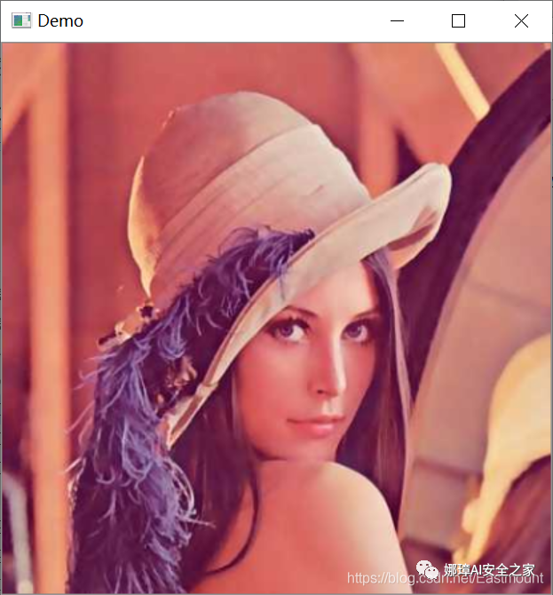
2. Channel merge
This function is the reverse operation of split() function, which synthesizes multiple arrays into an array of channels, so as to realize the merging of image channels. Its function prototype is as follows:
- dst = merge(mv[, dst]) – mv indicates the input array to be merged. All matrices must have the same size and depth – dst represents the output array with the same size and depth as mv[0]
The core code is as follows:
- m = cv2.merge([b, g, r])
# -*- coding:utf-8 -*-
import cv2
import numpy as np

#Read picture
img = cv2.imread("Lena.png")

#Split channel
b, g, r = cv2.split(img)

#Merge channel
m = cv2.merge([b, g, r])
cv2.imshow("Merge", m)

#Wait for display
cv2.waitKey(0)
cv2.destroyAllWindows()
The output results are as follows. It combines the color components of the split B, G and R channels, and then displays the combined image.
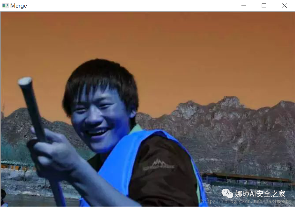
Note that if the [r,g,b] three channels are merged, the display is as follows, because OpenCV is read according to BGR.
- b, g, r = cv2.split(img)
- m = cv2.merge([r, g, b])
- cv2.imshow("Merge", m)
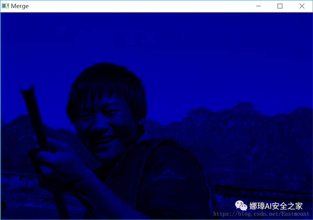
At the same time, different colors of the image can be extracted, and the B color channel can be extracted. If the G and B channels are set to 0, blue will be displayed. The code is as follows:
# -*- coding:utf-8 -*-
import cv2
import numpy as np

#Read picture
img = cv2.imread("test.jpg", cv2.IMREAD_UNCHANGED)
rows, cols, chn = img.shape

#Split channel
b = cv2.split(img)[0]
g = np.zeros((rows,cols),dtype=img.dtype)
r = np.zeros((rows,cols),dtype=img.dtype)

#Merge channel
m = cv2.merge([b, g, r])
cv2.imshow("Merge", m)

#Wait for display
cv2.waitKey(0)
cv2.destroyAllWindows()
The output results of the blue channel are as follows:
The core code and output results of green channel are as follows:
- rows, cols, chn = img.shape
- b = np.zeros((rows,cols), dtype=img.dtype)
- g = cv2.split(img)[1]
- r = np.zeros((rows,cols), dtype=img.dtype)
- m = cv2.merge([b, g, r])
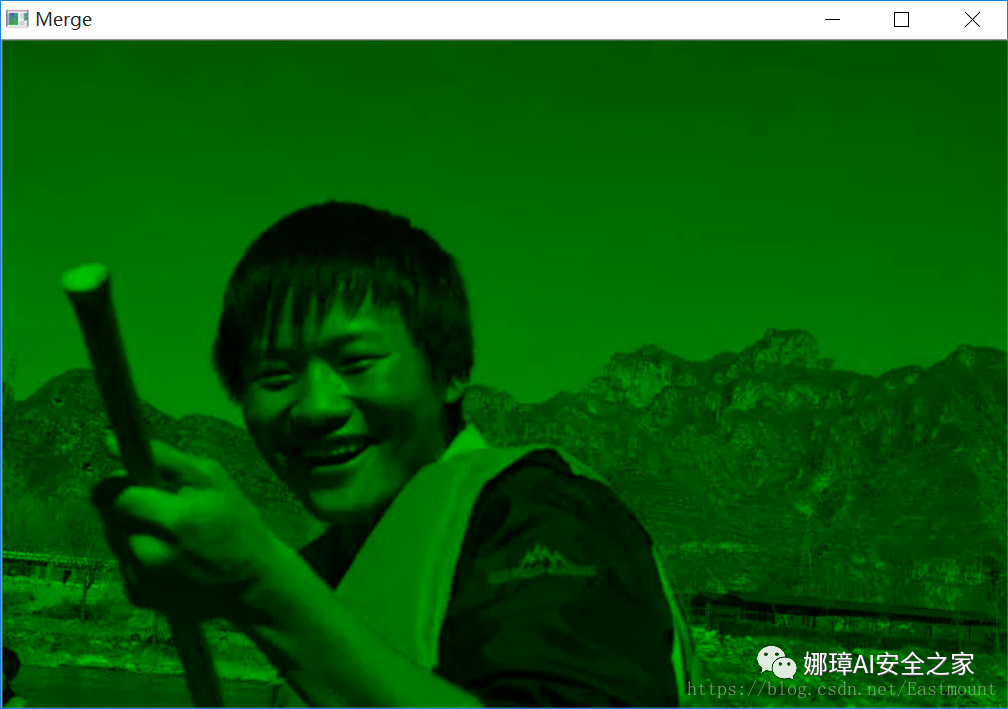
The red channel modification method is similar to the above.
4, Image type conversion
In daily life, most of the color images we see are RGB, but in the process of image processing, we often need to use gray image, binary image, HSV, HSI and other colors. Image type conversion refers to converting one type to another, such as color image to gray image and BGR image to RGB image. OpenCV provides conversion between more than 200 different types, of which the most commonly used include 3 types, as follows:
- cv2.COLOR_BGR2GRAY
- cv2.COLOR_BGR2RGB
- cv2.COLOR_GRAY2BGR
OpenCV provides the cvtColor() function to implement these functions. Its function prototype is as follows:
- dst = cv2.cvtColor(src, code[, dst[, dstCn]]) – src represents the input image and the original image requiring color space transformation – dst represents the output image, and its size and depth are consistent with src – code indicates the code or identification of the conversion – dstCn indicates the number of target image channels. When its value is 0, it is determined by src and code
The function is used to convert an image from one color space to another, where RGB refers to Red, Green and Blue, and an image is composed of these three channels; Gray indicates that there is only one channel of gray Value; HSV contains Hue, Saturation and Value channels. In OpenCV, common color space conversion identifiers include:
- CV_BGR2BGRA
- CV_RGB2GRAY
- CV_GRAY2RGB
- CV_BGR2HSV
- CV_BGR2XYZ
- CV_BGR2HLS
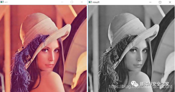
The following is the code that calls the cvtColor() function to grayscale the image.
#encoding:utf-8
import cv2
import numpy as np
import matplotlib.pyplot as plt

#Read picture
src = cv2.imread('Lena.png')

#Image type conversion
result = cv2.cvtColor(src, cv2.COLOR_BGR2GRAY)

#Display image
cv2.imshow("src", src)
cv2.imshow("result", result)

#Wait for display
cv2.waitKey(0)
cv2.destroyAllWindows()
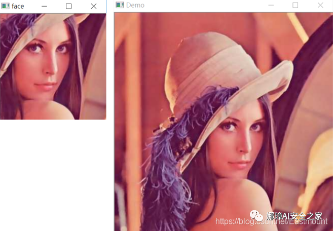
The output result is shown in the figure. It converts the color image on the left into the gray image on the right. For more gray conversion algorithms, refer to the subsequent articles.
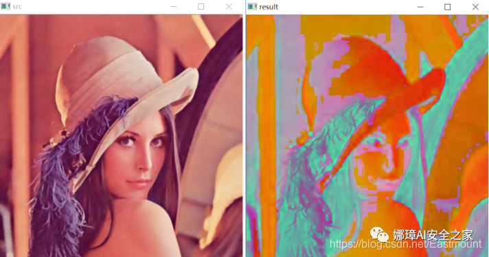
Similarly, you can call:
- grayImage = cv2.cvtColor(src, cv2.COLOR_BGR2HSV)
The core code converts the color image into HSV color space, as shown in the figure.
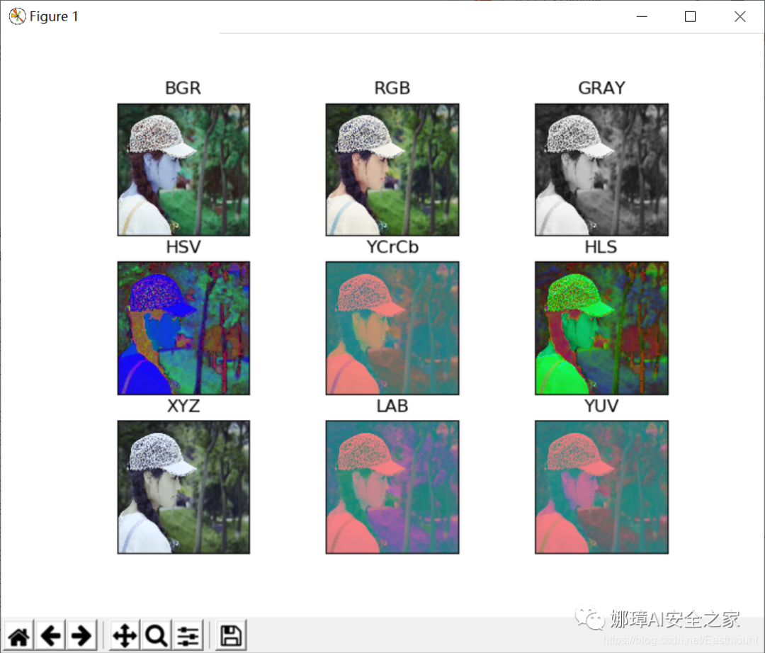
The following code compares nine common color spaces, including BGR, RGB, GRAY, HSV, YCrCb, HLS, XYZ, LAB and YUV, and circulates the processed images.
# -*- coding: utf-8 -*-
# By: Eastmount CSDN 2021-01-26
import cv2
import numpy as np
import matplotlib.pyplot as plt

#Read original image
img_BGR = cv2.imread('na.png')

#Convert BGR to RGB
img_RGB = cv2.cvtColor(img_BGR, cv2.COLOR_BGR2RGB)

#Grayscale processing
img_GRAY = cv2.cvtColor(img_BGR, cv2.COLOR_BGR2GRAY)

#BGR to HSV
img_HSV = cv2.cvtColor(img_BGR, cv2.COLOR_BGR2HSV)

#BGR to YCrCb
img_YCrCb = cv2.cvtColor(img_BGR, cv2.COLOR_BGR2YCrCb)

#BGR to HLS
img_HLS = cv2.cvtColor(img_BGR, cv2.COLOR_BGR2HLS)

#BGR to XYZ
img_XYZ = cv2.cvtColor(img_BGR, cv2.COLOR_BGR2XYZ)

#BGR to LAB
img_LAB = cv2.cvtColor(img_BGR, cv2.COLOR_BGR2LAB)

#BGR to YUV
img_YUV = cv2.cvtColor(img_BGR, cv2.COLOR_BGR2YUV)

#Call matplotlib to display the processing results
titles = ['BGR', 'RGB', 'GRAY', 'HSV', 'YCrCb', 'HLS', 'XYZ', 'LAB', 'YUV']
images = [img_BGR, img_RGB, img_GRAY, img_HSV, img_YCrCb,
          img_HLS, img_XYZ, img_LAB, img_YUV]
for i in range(9):
   plt.subplot(3, 3, i+1), plt.imshow(images[i], 'gray')
   plt.title(titles[i])
   plt.xticks([]),plt.yticks([])
plt.show()
The operation results are shown in the figure:
5, Summary
This is the end of this basic article. I hope the article will be helpful to you. If there are mistakes or deficiencies, please forgive me. This article starts with CSDN column, so as to help more students, update the official account number and cheer up!
- 1, Get image properties
- 2, Get ROI region of interest
- 3, Image channel processing
- 4, Image type conversion
reference:
- [1] Luo Zijiang. Image processing in Python [M]. Science Press, 2020
- [2] https://blog.csdn.net/eastmount/category_9278090.html
- [3] Gonzalez. Digital image processing (3rd Edition) [M]. Electronic Industry Press, 2013
- [4] Ruan Qiuqi. Digital image processing (3rd Edition) [M]. Electronic Industry Press, 2008
- [5] Mao Xingyun, Leng Xuefei. Introduction to OpenCV3 programming [M]. Electronic Industry Press, 2015
- [6] Zhang Zheng. Digital image processing and machine vision -- implementation with Visual C + + and Matlab
- [6] Netease cloud classroom_ Gordon education. Python+OpenCV image processing