Python artificial intelligence VI. basic usage of Tensorboard visualization and neural network rendering

After a busy week, I had a rest in the evening and then shared AI knowledge. The author of this series will explain Python deep learning, neural network and artificial intelligence. I hope you like it.

The previous article explained how TensorFlow creates a regression neural network and Optimizer optimizer; This article will explain the basic usage of Tensorboard visualization in detail, and draw the changes of the parameters of the whole neural network, training and learning. This article mainly combines the author's previous blog, "don't bother God" video and AI experience. Later, more Python AI cases and applications will be explained in depth.

Basic articles, I hope to help you. If there are errors or deficiencies in the articles, please Haihan ~ at the same time, I am also a rookie of artificial intelligence. I hope you can grow up with me in this stroke by stroke blog.

Article directory:

1, First acquaintance with tensorboard
2, tensorboard drawing graph
3, tensorboard visual neural network learning process
4, Summary

Code download address:

https://github.com/eastmountyxz/ AI-for-TensorFlow
https://github.com/eastmountyxz/ AI-for-Keras

1, First acquaintance with tensorboard

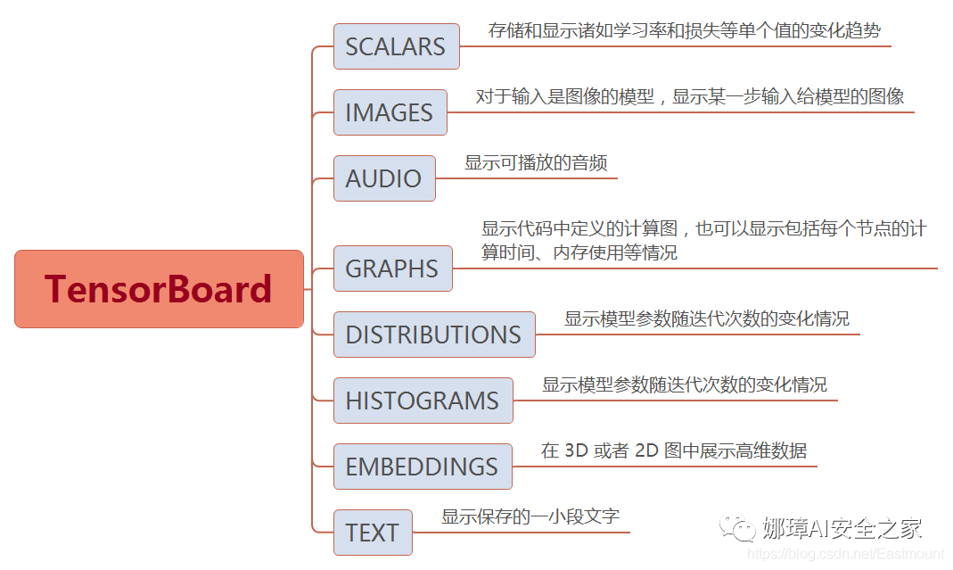
Tensorboard is a utility provided by TensorFlow. It can graphically display Graph to help developers understand, debug and optimize TensorFlow programs. The main panels of tensorboard are shown in the figure below:

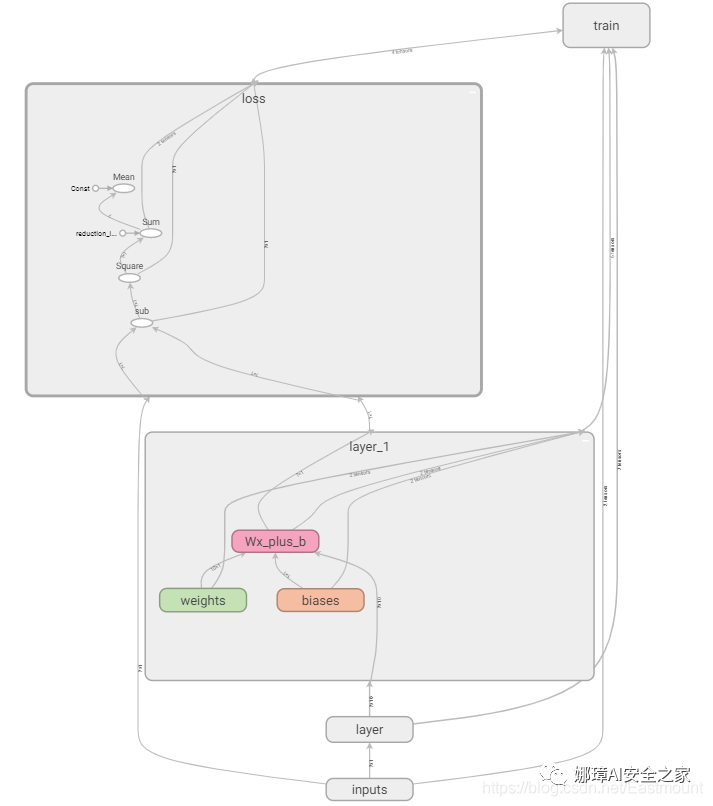
Many times, we write neural networks, but we don't have a good visual display. This article will share how to visualize the neural network through the Tensorboard provided by TensorFlow itself. Through it, you can intuitively see the whole neural network or the framework structure of TensorFlow, as shown in the figure below.

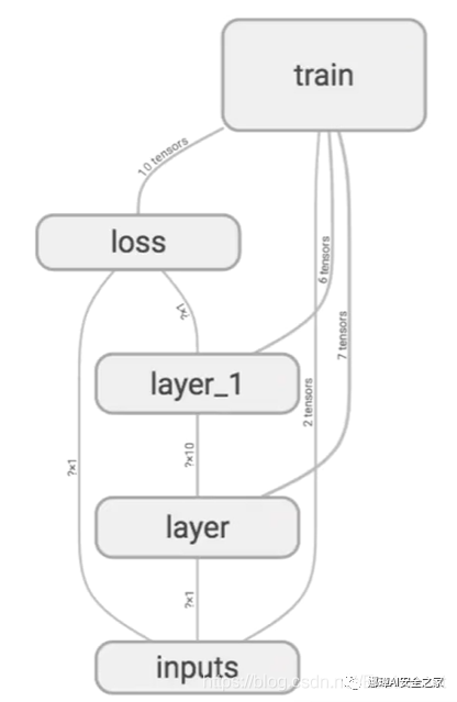
This structure is roughly divided into input layer, two hidden layers and calculation error loss.

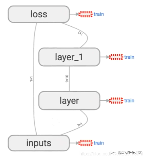
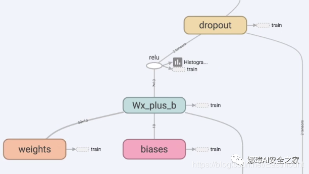
Click to expand a hidden layer, and you can see weight Wights, deviation bias and calculation method Wx_plus_b and excitation function Relu, etc. We can intuitively see how TensorFlow's data flows to the neural network.

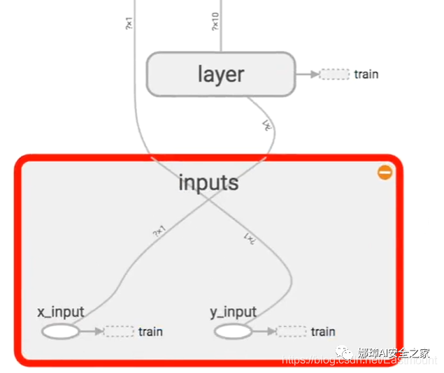
At the same time, inputs include x_input and y_input two values.

Next, we begin to write the visualization function of neural network. Here, we still use the code of the last lesson, which realizes a regression neural network through TensorFlow, and fits a curve close to the scatter point through continuous learning.

# -*- coding: utf-8 -*-
"""
Created on Mon Dec 16 21:34:11 2019
@author: xiuzhang CSDN Eastmount
"""
import tensorflow as tf
import numpy as np
import matplotlib.pyplot as plt

#---------------------------------Define neural layer---------------------------------
# Function: input variable input size output size excitation function default None
def add_layer(inputs, in_size, out_size, activation_function=None):
    # The weight is a random variable matrix
    Weights = tf.Variable(tf.random_normal([in_size, out_size]))    #Row * column
    # The initial value of the defined offset is increased by 0.1, which changes in each training
    biases = tf.Variable(tf.zeros([1, out_size]) + 0.1)             #1 row and multiple columns
    # Defines the predicted value of the calculated matrix multiplication
    Wx_plus_b = tf.matmul(inputs, Weights) + biases
    # Activate operation
    if activation_function is None: 
        outputs = Wx_plus_b
    else:
        outputs = activation_function(Wx_plus_b)
    return outputs

#---------------------------------Construction data---------------------------------
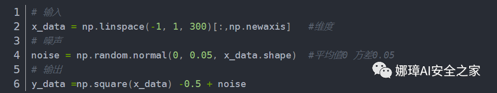
# input
x_data = np.linspace(-1, 1, 300)[:,np.newaxis]   #dimension
# Noise
noise = np.random.normal(0, 0.05, x_data.shape)  #Mean value 0, variance 0.05
# output
y_data =np.square(x_data) -0.5 + noise

# Set the passed in values xs and ys
xs = tf.placeholder(tf.float32, [None, 1]) #x_data passed in to xs
ys = tf.placeholder(tf.float32,[None, 1]) #y_data passed in to ys

#---------------------------------Defining neural networks---------------------------------
# Hidden layer
L1 = add_layer(xs, 1, 10, activation_function=tf.nn.relu) #Excitation function
# Output layer
prediction = add_layer(L1, 10, 1, activation_function=None)

#------------------------------Define loss and initialization-------------------------------
# Average error between predicted value and real value - > sum - > square (real value - predicted value)
loss = tf.reduce_mean(tf.reduce_sum(tf.square(ys - prediction), 
                     reduction_indices=[1]))
# The training efficiency is usually less than 1, which can be set to 0.1 for comparison
train_step = tf.train.GradientDescentOptimizer(0.1).minimize(loss) #Reduce error

# initialization
init = tf.initialize_all_variables()
# function
sess = tf.Session()
sess.run(init)

#---------------------------------Visual analysis---------------------------------
# Define picture box
fig = plt.figure()
ax = fig.add_subplot(1,1,1)
# Scatter diagram
ax.scatter(x_data, y_data)
# Continuous display
plt.ion()
plt.show()

#---------------------------------Neural network learning---------------------------------
# Learn 1000 times
n = 1
for i in range(1000):
    # train
    sess.run(train_step, feed_dict={xs:x_data, ys:y_data}) #Assume all data x_data
    # As long as the output result passes through place_ To run holder, you need to pass in parameters
    if i % 50==0:
        #print(sess.run(loss, feed_dict={xs:x_data, ys:y_data}))
        try:
            # Ignore the first error and subsequently remove the first line segment of lines
            ax.lines.remove(lines[0])
        except Exception:
            pass
        # forecast
        prediction_value = sess.run(prediction, feed_dict={xs:x_data})
        # Set the line width to 5 red
        lines = ax.plot(x_data, prediction_value, 'r-', lw=5) 
        # suspend
        plt.pause(0.1)
        # Save picture
        name = "test" + str(n) + ".png"
        plt.savefig(name)
        n =  n + 1

The output results are shown in the figure below. From the earliest unreasonable figure to the later basic fitting, the loss error is decreasing, indicating that the real value and predicted value of the neural network are constantly updated and close, and the neural network operates normally.

2, tensorboard drawing graph

Next, we use Tensorboard for visual training, and modify the above code as follows.

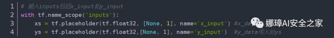
The first step is to modify from input and call tf.name_scope() sets the input layer name and adds names to the passed in values xs and ys. The entire inputs include x_input and y_input.

tf.name_ The actual functions of the scope () namespace are as follows:

In a tf.name_ All objects and operations are defined in the area specified by scope(). The area name of the named area will be added to their "name" attribute to distinguish which area the object belongs to;
Different objects and operations are placed by tf.name_ In the area specified by scope (), it is convenient to show a clear logical diagram in the tensorboard, which is particularly important in complex diagrams.

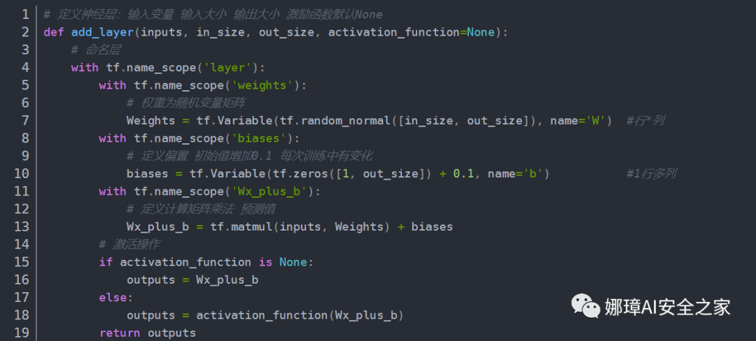
Step 2: modify add_layer() function through tf.name_ The scope () function names regions and variables.

Here, use with tf.name_ The scope ('layer ') code names the area. We regard the layer layer as a framework, corresponding to the layer area of the previous visual graphics. Note that the excitation function is not named because it will have a name by default. For example, if "relu" is selected, its name is "relu".

The third step is to define the layer name. Every time you add a layer, it will add a corresponding frame, which is the layer named in the second step.

Step 4, then through tf.name_ The scope () function defines the loss and train frameworks.

Step 5: initialization and file writing.

The complete code at this time is as follows:

# -*- coding: utf-8 -*-
"""
Created on Tue Dec 17 10:51:40 2019
@author: xiuzhang CSDN Eastmount
"""
import tensorflow as tf

#---------------------------------Define neural layer---------------------------------
# Function: input variable input size output size excitation function default None
def add_layer(inputs, in_size, out_size, activation_function=None):
    # Naming layer
    with tf.name_scope('layer'):
        with tf.name_scope('weights'):
            # The weight is a random variable matrix
            Weights = tf.Variable(tf.random_normal([in_size, out_size]), name='W')  #Row * column
        with tf.name_scope('biases'):
            # The initial value of the defined offset is increased by 0.1, which changes in each training
            biases = tf.Variable(tf.zeros([1, out_size]) + 0.1, name='b')           #1 row and multiple columns
        with tf.name_scope('Wx_plus_b'):
            # Defines the predicted value of the calculated matrix multiplication
            Wx_plus_b = tf.matmul(inputs, Weights) + biases
        # Activate operation
        if activation_function is None: 
            outputs = Wx_plus_b
        else:
            outputs = activation_function(Wx_plus_b)
        return outputs

#-----------------------------Set the passed in values xs and ys-------------------------------
# Input includes x_input and y_input
with tf.name_scope('inputs'):
    xs = tf.placeholder(tf.float32, [None, 1], name='x_input') #x_data passed in to xs
    ys = tf.placeholder(tf.float32,[None, 1], name='y_input')  #y_data passed in to ys

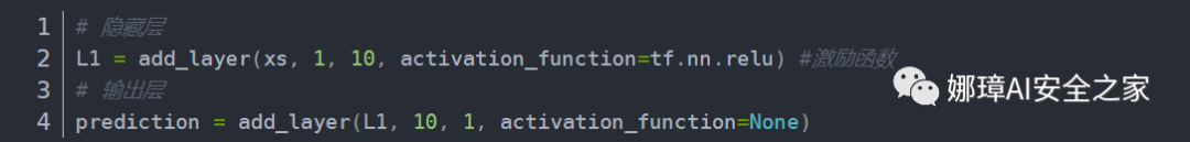
#---------------------------------Defining neural networks---------------------------------
# Hidden layer
L1 = add_layer(xs, 1, 10, activation_function=tf.nn.relu) #Excitation function
# Output layer
prediction = add_layer(L1, 10, 1, activation_function=None)

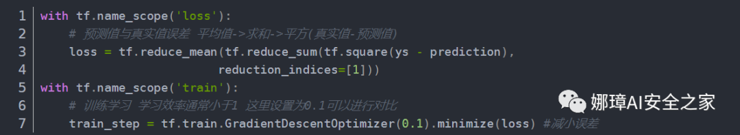
#------------------------------Define loss and train-------------------------------
with tf.name_scope('loss'):
    # Average error between predicted value and real value - > sum - > square (real value - predicted value)
    loss = tf.reduce_mean(tf.reduce_sum(tf.square(ys - prediction), 
                         reduction_indices=[1]))
with tf.name_scope('train'):
    # The training efficiency is usually less than 1, which can be set to 0.1 for comparison
    train_step = tf.train.GradientDescentOptimizer(0.1).minimize(loss) #Reduce error

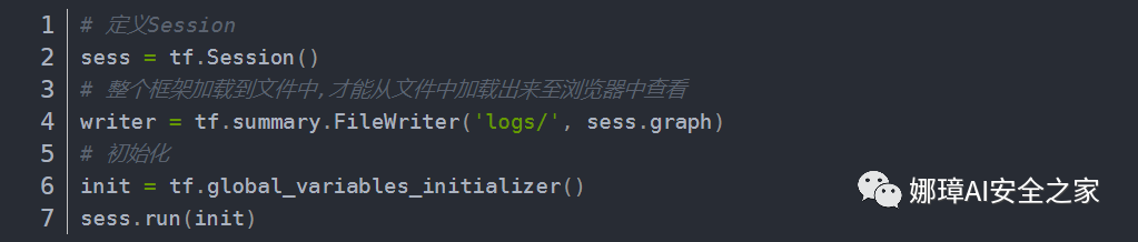
#------------------------------Initialization and file write operations-------------------------------
# Define Session
sess = tf.Session()
# The whole frame can only be loaded from the file and viewed in the browser after being loaded into the file
writer = tf.summary.FileWriter('logs/', sess.graph)
# initialization
init = tf.global_variables_initializer()
sess.run(init)

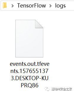
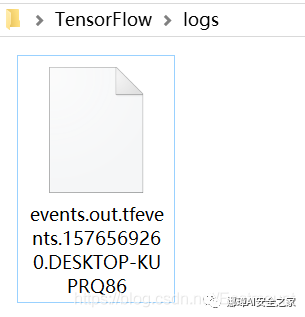
We try to run the code. At this time, a new "logs" folder and events file will be created in the Python file directory, as shown in the following figure.

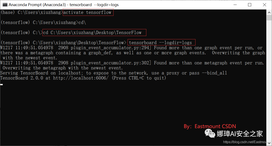
Next, try opening it. First, call Anaconda Prompt and activate TensorFlow. Then go to the directory of events file and call the command "tensorboard --logdir=logs" to run, as shown in the figure below. Note that you only need to guide to the folder, and it will automatically index your files.

activate tensorflow
cd\
cd C:\Users\xiuzhang\Desktop\TensorFlow
tensorboard --logdir=logs

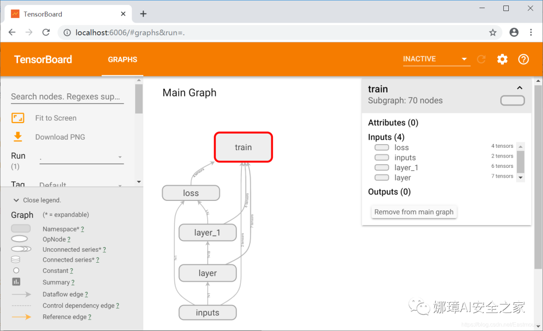
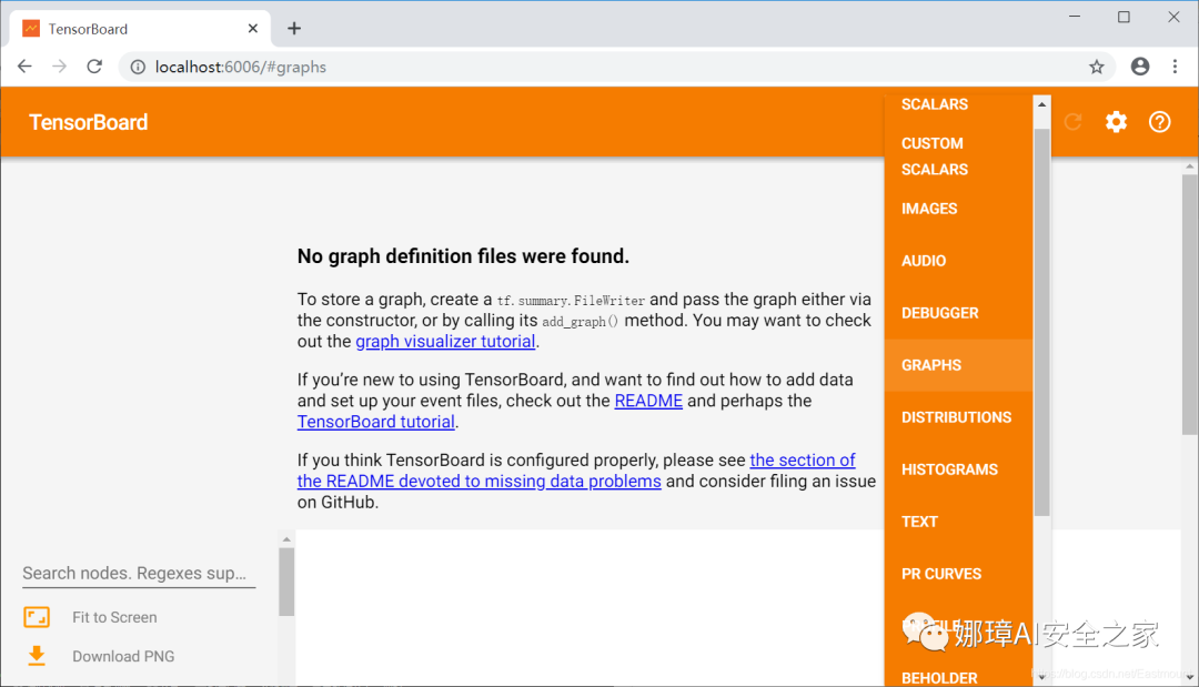
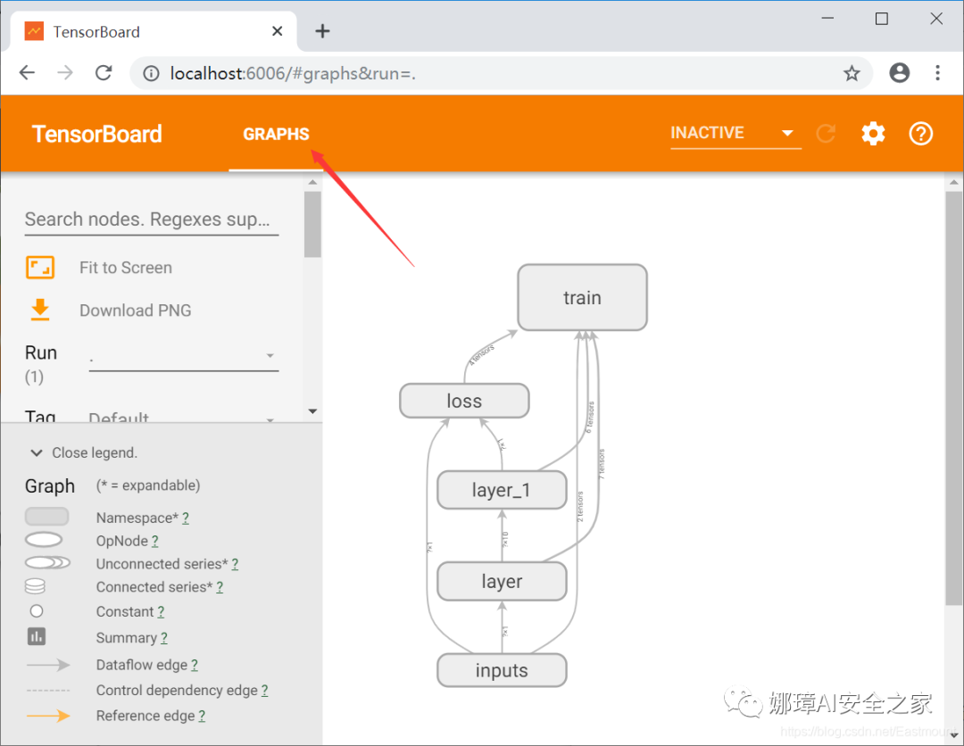
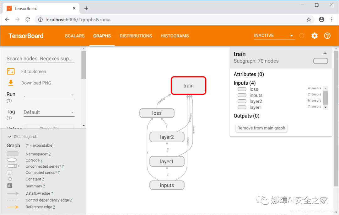
Visit the web address at this time“ http://localhost:6006/ ”, select "Graphs". After running, as shown in the figure below, our neural network appears.

Double click each layer to see the details, such as layer, as shown in the following figure, including weight, offset and calculation function.

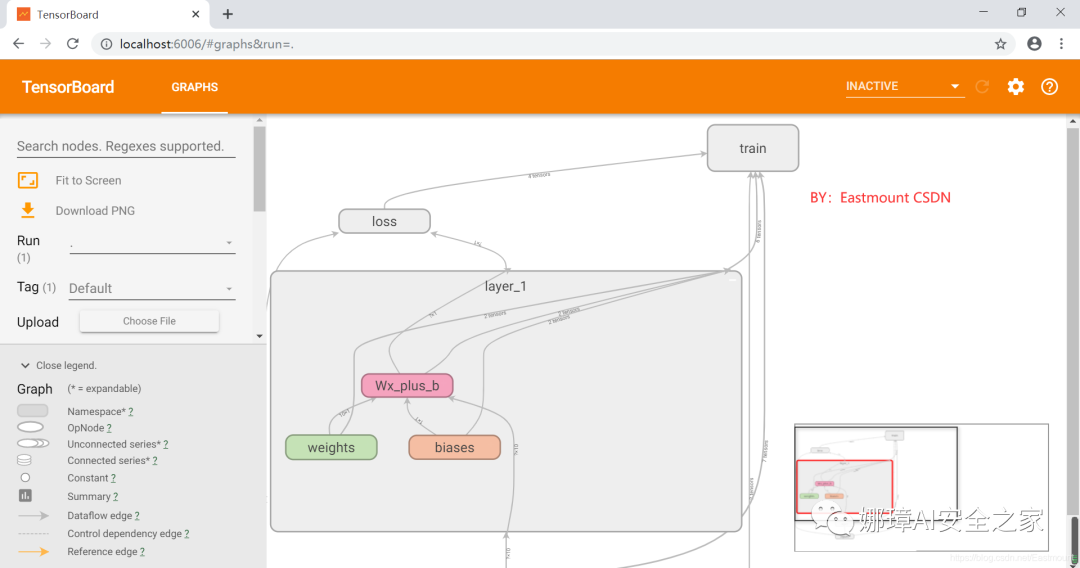
For another example, click the loss calculation function, and its processing flow is shown in the figure below.

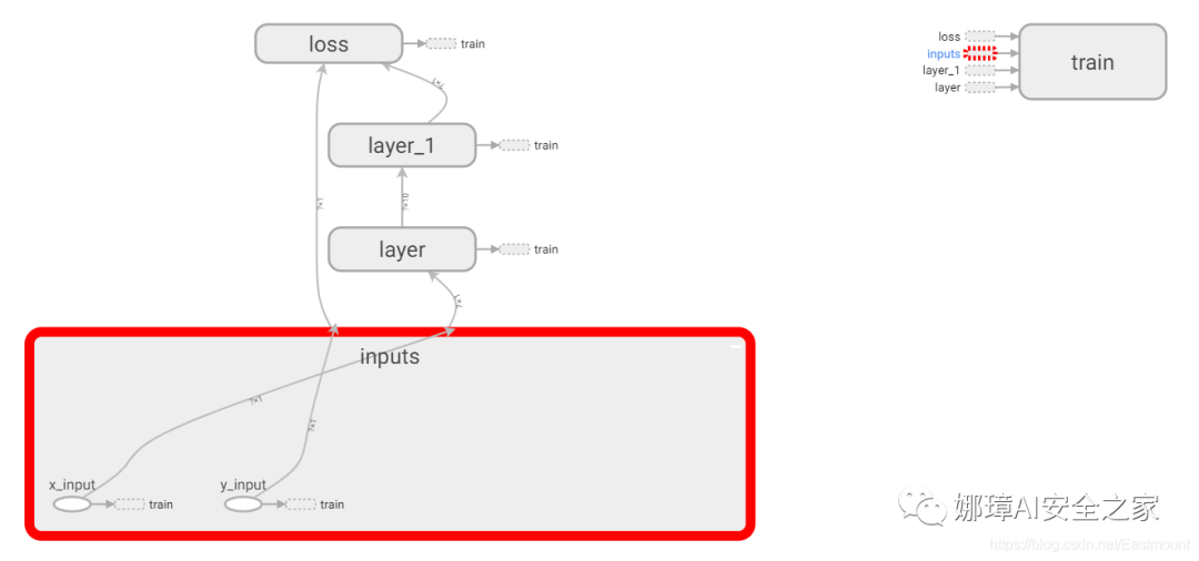
Usually, we will put the train part aside, select "train", and then right-click "Remove from main graph".

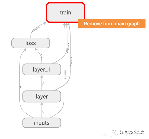
The display results at this time are shown in the following figure. At the same time, the input layer inputs include x_input and y_input.

PS: "No graph definition files were found" will be displayed when visualized with tensorboard, which is likely to be a path error. You should pay attention to naming folders in English and avoid spaces.

3, tensorboard visualization

Next, we use Tensorboard for visual training and modify the above code as follows. At this time, the neural network only has Graph function. Next, we try to visually display its DISTRIBUTIONS, HISTOGRAMS, EVENTS and other panels.

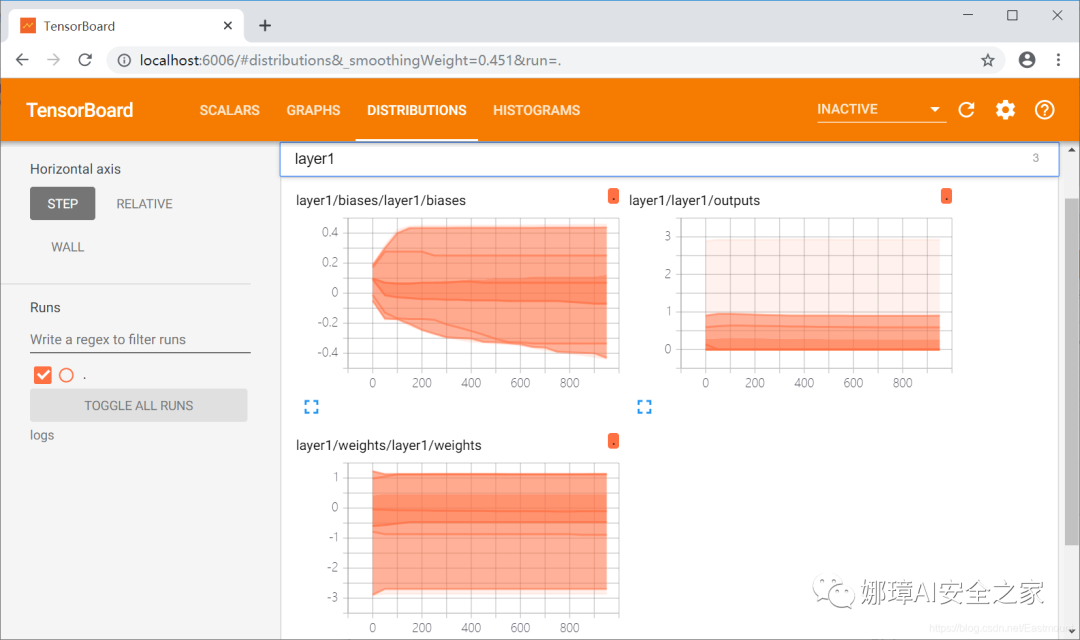
DISTRIBUTIONS is the whole training process, showing the changes of Weights, outputs and bias of Layer1.

In EVENTS, the error loss can also be displayed.

Then start to explain the code.

The first step is to write code to construct data.

First, import the expansion pack numpy.

import numpy as np

Then three variables, input, noise and output, are constructed.

Step 2: add the name of the drawing display in the add_layer() function, as shown in the upper left corner of the figure below.

Amend as follows:

1. Customize a variable layer_name whose value is the parameter n_layer passed in from the add_layer() function.
2. The function add_layer(inputs, in_size, out_size, n_layer, activation_function=None) adds the parameter n_layer, which is the name of the neural layer.
3. Modify tf.name_scope(layer_name), and the passed value is layer_name.
4. Use the tf.summary.histogram() function to define the name of the upper left corner of the graph, including weights, bias and outputs. Some TensorFlow versions call the tf.histogram_summary() function.

The modified code is as follows:

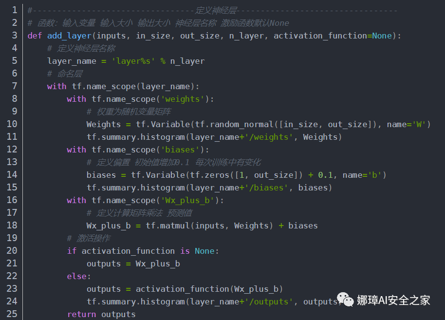
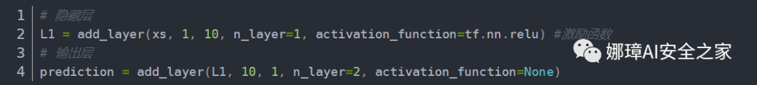
The third step is to modify the code defining the neural network, add the parameter n_layer, and set it to layer 1 and layer 2.

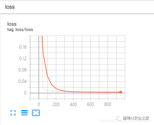
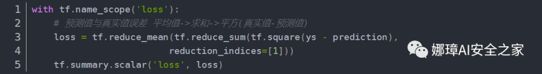
The fourth step is to visualize the change of loss. It is displayed in EVENTS\SCALARS in the form of stock and implemented by calling tf.scalar_summary() function. If the loss is decreasing, it indicates that the neural network has learned something.

Step 5: merge all the summaries together.

# Merge all summaries
merged = tf.summary.merge_all()

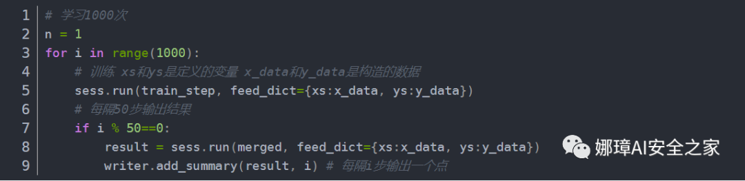
Step 6, write the neural network learning process, and output the results every 50 steps.

The final complete code is as follows:

# -*- coding: utf-8 -*-
"""
Created on Tue Dec 17 10:51:40 2019
@author: xiuzhang CSDN Eastmount
"""
import tensorflow as tf
import numpy as np

#---------------------------------Define neural layer---------------------------------
# Function: input variable input size output size neural layer name excitation function default None
def add_layer(inputs, in_size, out_size, n_layer, activation_function=None):
    # Define neural layer name
    layer_name = 'layer%s' % n_layer
    # Naming layer
    with tf.name_scope(layer_name):
        with tf.name_scope('weights'):
            # The weight is a random variable matrix
            Weights = tf.Variable(tf.random_normal([in_size, out_size]), name='W')  #Row * column
            tf.summary.histogram(layer_name+'/weights', Weights)
        with tf.name_scope('biases'):
            # The initial value of the defined offset is increased by 0.1, which changes in each training
            biases = tf.Variable(tf.zeros([1, out_size]) + 0.1, name='b')           #1 row and multiple columns
            tf.summary.histogram(layer_name+'/biases', biases)
        with tf.name_scope('Wx_plus_b'):
            # Defines the predicted value of the calculated matrix multiplication
            Wx_plus_b = tf.matmul(inputs, Weights) + biases
        # Activate operation
        if activation_function is None: 
            outputs = Wx_plus_b
        else:
            outputs = activation_function(Wx_plus_b)
            tf.summary.histogram(layer_name+'/outputs', outputs)
        return outputs

#---------------------------------Construction data-----------------------------------
# input
x_data = np.linspace(-1, 1, 300)[:,np.newaxis]   #dimension
# Noise
noise = np.random.normal(0, 0.05, x_data.shape)  #Mean value 0, variance 0.05
# output
y_data =np.square(x_data) -0.5 + noise

#-----------------------------Set the passed in values xs and ys-------------------------------
# Input inputs include x_input and y_input
with tf.name_scope('inputs'):
    xs = tf.placeholder(tf.float32, [None, 1], name='x_input') #x_data passed in to xs
    ys = tf.placeholder(tf.float32,[None, 1], name='y_input')  #y_data passed to ys

#---------------------------------Defining neural networks---------------------------------
# Hidden layer
L1 = add_layer(xs, 1, 10, n_layer=1, activation_function=tf.nn.relu) #Excitation function
# Output layer
prediction = add_layer(L1, 10, 1, n_layer=2, activation_function=None)

#------------------------------Define loss and train-------------------------------
with tf.name_scope('loss'):
    # Average error between predicted value and real value - > sum - > square (real value - predicted value)
    loss = tf.reduce_mean(tf.reduce_sum(tf.square(ys - prediction), 
                         reduction_indices=[1]))
    tf.summary.scalar('loss', loss)
    
with tf.name_scope('train'):
    # The training efficiency is usually less than 1, which can be set to 0.1 for comparison
    train_step = tf.train.GradientDescentOptimizer(0.1).minimize(loss) #Reduce error

#------------------------------Initialization and file write operations-------------------------------
# Define Session
sess = tf.Session()
# Merge all summaries
merged = tf.summary.merge_all()

# The whole frame can only be loaded from the file and viewed in the browser after being loaded into the file
writer = tf.summary.FileWriter('logs/', sess.graph)
# initialization
init = tf.global_variables_initializer()
sess.run(init)

#---------------------------------Neural network learning---------------------------------
# Learn 1000 times
n = 1
for i in range(1000):
    # Training xs and ys are defined variables, and x_data and y_data are constructed data
    sess.run(train_step, feed_dict={xs:x_data, ys:y_data})
    # Output results every 50 steps
    if i % 50==0:
        result = sess.run(merged, feed_dict={xs:x_data, ys:y_data})
        writer.add_summary(result, i) # Output a point every i steps

Run the code to generate a new output file.

Enter the command "tensorboard --logdir=logs" in Anaconda Prompt, and then call the browser to view the newly generated graphics, as shown in the following figure.

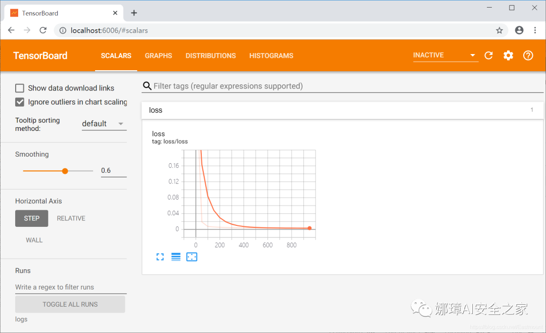
At this time, the visual graph of loss will be displayed in SCALARS. It is found that the error is decreasing, the neural network continues to learn, and the fitting curve is also improving.

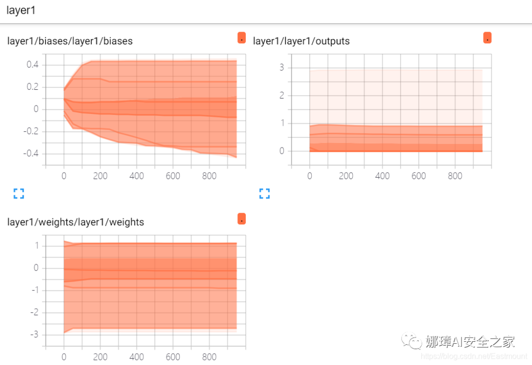
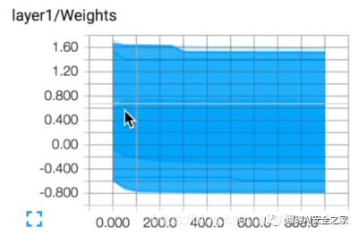
Layer1 displayed in DISTRIBUTIONS is shown in the following figure. The darker the color, the more values in this area. A point will be generated every 50 steps, including bias, weights and outputs.

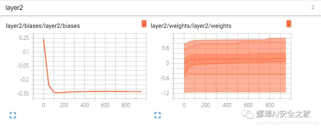
Layer2 displayed by DISTRIBUTIONS is shown in the following figure

HISTOGRAMS is displayed as shown in the following figure:

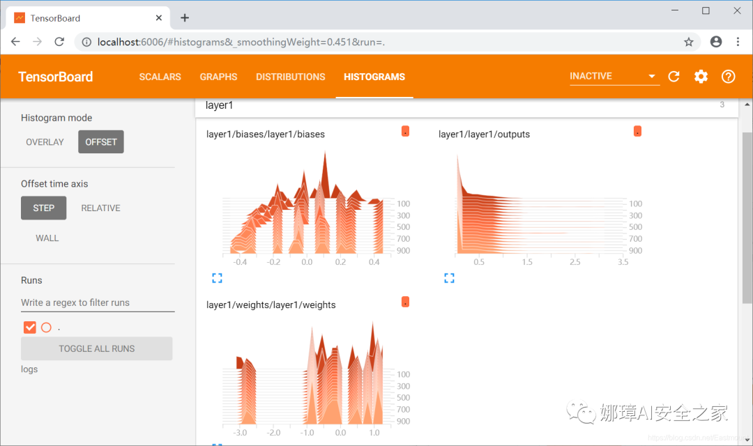
Histograms panel and distributions panel display the changes of model parameters with the number of iterations. Distributions panel is used to display the changes of parameters in the network with the increase of training steps, such as the distribution of weights. Histograms panel and distributions display the same data in different ways, which is the stacking of frequency histograms.

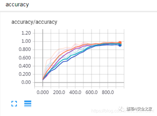
With the in-depth sharing of the article, the visual comparison of different neural networks will be explained in combination with cases and evaluation indicators, such as Accuracy, Precision, Recall, F-measure, etc.

4, Summary

At this point, this article ends. The main content is to use Tensorboard to observe our neural network. I'm really busy. I hope this basic article will help you. If there are errors or deficiencies in the article, please Haihan ~ as a rookie of artificial intelligence, I hope I can make continuous progress and deepen, and apply it to image recognition and network in the future Safety, confrontation and other fields, come on!

References, thank you for your articles and videos. I recommend you to follow Mr. Mo fan. He is my introductory teacher of artificial intelligence.

[1] Introduction to neural networks and machine learning - author's article
[2] Stanford machine learning video Professor NG: https://class.coursera.org/ml/class/index
[3] Book "artificial intelligence in game development"
[4] Netease cloud don't bother teacher video (strong push): https://study.163.com/course/courseLearn.htm?courseId=1003209007
[5] Neural network excitation function - deep learning
[6] tensorflow Architecture - NoMorningstar
[7] Tensorflow 2.0 introduction to low level api - GumKey
[8] Fundamentals of tensorflow - kk123k
[9] tensorboard tutorial - 77 ah
[10] The use of Tensorboard, the visualization tool of tensorflow -- the use of scalar -- the freedom of self-discipline

Posted by Grant Cooper on Thu, 02 Dec 2021 11:38:19 -0800

Programmer Group

Python artificial intelligence VI. basic usage of Tensorboard visualization and neural network rendering

1, First acquaintance with tensorboard

2, tensorboard drawing graph

3, tensorboard visualization

4, Summary

Hot Keywords