0 Introduction

Today, the senior introduces a machine vision project to you

Image correction based on machine vision (taking license plate recognition as an example)

Bi design help, problem opening guidance, technical solutions
🇶746876041

1 Introduction to ideas

At present, the license plate recognition system can be seen everywhere at the door of each community, and the recognition effect seems to be OK. After consulting the data, it is found that the whole process can be subdivided into four parts: license plate location, distortion correction, license plate segmentation and content recognition. This essay mainly introduces two parts: license plate location and distortion correction, which are realized by opencv in python environment.

1.1 license plate location

At present, the mainstream license plate location methods can be divided into two categories: one is based on the background color feature of license plate; Another method is based on the contour shape feature of license plate. Based on color features can be divided into two categories: one in RGB space and the other in HSV space. After testing, it is found that the effect of using any method alone is not ideal. At present, it is common to use several positioning methods at the same time, or use one recognition and the other verification. In this paper, the license plate is located mainly through color features, mainly based on the H component of HSV space, supplemented by the R component and B component of RGB space, and then the length width ratio of the license plate is used to eliminate interference.

1.2 distortion correction

In the process of license plate image acquisition, the camera lens is usually not perpendicular to the license plate, so the license plate in the image to be recognized will be distorted to a certain extent, which brings some difficulties to the subsequent license plate content recognition. Therefore, it is necessary to correct the distortion of the license plate to eliminate the adverse effects of distortion.

2 code implementation

2.1 license plate location

2.1.1 select suspicious areas through color features

The images of the license plate under different lighting environments are taken, the background color is intercepted, and the channel separation and color space conversion are carried out by opencv. After the test, the following characteristics of the background color of the license plate are summarized:

• (1) In HSV space, the value of H component usually hovers around 115, and the s component and V component vary greatly due to different illumination (the value range of H component in opencv is 0 to 179, not 0 to 360 in iconography; the value range of S component and V component is 0 to 255);

• (2) In RGB space, the R component is usually small, generally below 30, the B component is usually large, generally above 80, and the G component fluctuates greatly;

• (3) In the HSV space, the image is filled with light and saturated, that is, the S component and V component of the image are set to 255, and then the color space is converted from HSV space to RGB space. It is found that all R components become 0 and all B components become 255 (this operation will introduce large interference and will not be used later).

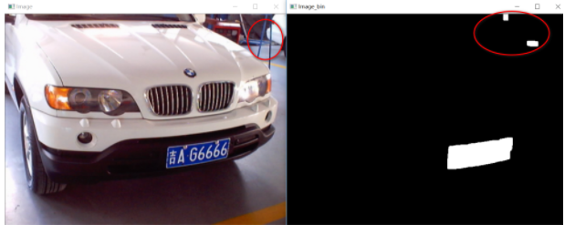
According to the above features, the suspicious license plate area can be preliminarily screened. Then, the gray image is operated, and the pixel value of the suspicious position is set to 255 and the pixel value of other positions is set to 0, that is, the image is binarized according to the features. In the binarized image, the suspicious area is represented by white and other areas are black. Then, the image can be further processed through expansion and corrosion .

for i in range(img_h):
    for j in range(img_w):
        # Ordinary blue license plate, while excluding the interference of transparent reflective materials
        if ((img_HSV[:, :, 0][i, j]-115)**2 < 15**2) and (img_B[i, j] > 70) and (img_R[i, j] < 40):
            img_gray[i, j] = 255
        else:
            img_gray[i, j] = 0

2.1.2 find the peripheral contour of the license plate

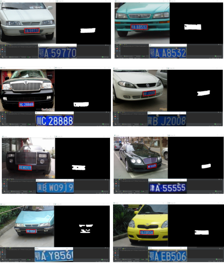
After selecting the suspicious area and binarizing the image, generally, only the pixel color of the license plate position in the image is white, but there will be some noise in some special cases. As shown in the above figure, because there is a blue bracket in the upper right corner of the image, which is consistent with the color characteristics of the license plate, it is also recognized as a license plate, which introduces noise.

Through observation, it can be found that there are great differences between the license plate area and noise, and the characteristics of the license plate area are obvious:

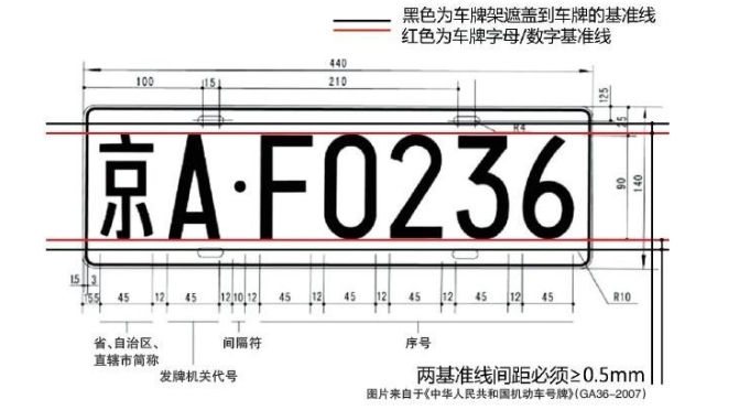
• (1) According to the shape of China's conventional license plate, the shape of the license plate is a flat rectangle, and the length width ratio is about 3:1;

• (2) The area of the license plate is much larger than the noise area, which is generally the largest white area in the image.

You can find the outline of the white area in the binarized image through the cv2.findContours() function.

Note: in opencv2 and opencv4, there are two return values of cv2.findContours(), while in opencv3, there are three return values. Depending on the opencv version, the code writing method will also be different.

# Detect all outer contours, leaving only four vertices of the rectangle
# opencv4.0, opencv2.x
contours, _ = cv2.findContours(img_bin, cv2.RETR_LIST, cv2.CHAIN_APPROX_SIMPLE)
# opencv3.x
_, contours, _ = cv2.findContours(img_bin, cv2.RETR_LIST, cv2.CHAIN_APPROX_SIMPLE)

Here, because there are three white areas (license plate and two noises) in the binary image, the return value contours is a list with a length of 3. The list contains three arrays, and each array stores the contour information of a white area. The shape of each array is (n, 1, 2), that is, each array stores the coordinates of n points on the contour of the white area.

At present, we have obtained three array s, that is, three groups of contour information, but we do not know which is the group of contour information corresponding to the license plate area. At this time, we can filter the contour of the license plate area according to the above characteristics of the license plate.

#Shape and size screening verification
det_x_max = 0
det_y_max = 0
num = 0
for i in range(len(contours)):
    x_min = np.min(contours[i][ :, :, 0])
    x_max = np.max(contours[i][ :, :, 0])
    y_min = np.min(contours[i][ :, :, 1])
    y_max = np.max(contours[i][ :, :, 1])
    det_x = x_max - x_min
    det_y = y_max - y_min
    if (det_x / det_y > 1.8) and (det_x > det_x_max ) and (det_y > det_y_max ):
        det_y_max = det_y
        det_x_max = det_x
        num = i
# Get the contour point set of the most suspicious area
points = np.array(contours[num][:, 0])

The shape of the final points is (n, 2), which stores the coordinates of n points, which are distributed on the edge of the license plate

2.1.3 location of license plate area

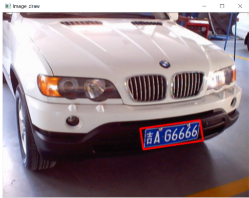
After obtaining the point set on the contour of the license plate, you can use CV2. Minaarearect() to obtain the minimum circumscribed rectangle of the point set. The return value rect contains the center point coordinates, height, width, inclination angle and other information of the rectangle. You can use cv2.boxPoints() to obtain the coordinates of the four vertices of the rectangle.

# Obtain the minimum circumscribed matrix, center point coordinates, width, height and rotation angle
rect = cv2.minAreaRect(points)
# Gets the four vertices of a rectangle, floating point
box = cv2.boxPoints(rect)
# Rounding
box = np.int0(box)

However, we do not know which vertex of the rectangle these four coordinate points correspond to, so we can not make full use of these coordinate information.

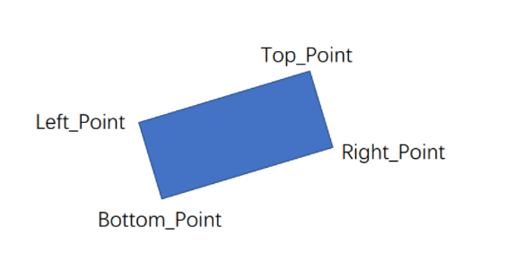
Starting from the size characteristics of coordinate values, the four coordinates can be matched with the four vertices of the rectangle: in the opencv coordinate system, the smallest ordinate is top_point, the largest ordinate is bottom_point, the smallest abscissa is left_point, and the largest abscissa is right_point.

# Get four vertex coordinates
left_point_x = np.min(box[:, 0])
right_point_x = np.max(box[:, 0])
top_point_y = np.min(box[:, 1])
bottom_point_y = np.max(box[:, 1])

left_point_y = box[:, 1][np.where(box[:, 0] == left_point_x)][0]
right_point_y = box[:, 1][np.where(box[:, 0] == right_point_x)][0]
top_point_x = box[:, 0][np.where(box[:, 1] == top_point_y)][0]
bottom_point_x = box[:, 0][np.where(box[:, 1] == bottom_point_y)][0]
# Up, down, left and right coordinates
vertices = np.array([[top_point_x, top_point_y], [bottom_point_x, bottom_point_y], [left_point_x, left_point_y], [right_point_x, right_point_y]])

2.2 distortion correction

2.2.1 vertex location of license plate after distortion

In order to realize the distortion correction of license plate, the position relationship of corresponding points before and after distortion must be found.

It can be seen that the rectangular license plate becomes a parallelogram after distortion, so the license plate contour does not match the obtained rectangular contour. However, with the four vertex coordinates of the rectangle, the four vertex coordinates of the parallelogram license plate can be obtained through a simple geometric similarity relationship.

In this example, the four vertices of the parallelogram and the four vertices of the rectangle have the following relationship: rectangular vertex Top_Point,Bottom_Point and parallelogram vertex new_top_point,new_bottom_point coincident, rectangular vertex top_ Abscissa of point and parallelogram vertex NEW_ right_ The abscissa of point is the same, and the rectangular vertex bottom_ Abscissa of point and parallelogram vertex NEW_ left_ The abscissa of point is the same.

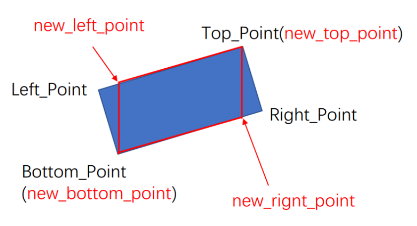
But in fact, due to different shooting angles, there may be two different distortions. The specific distortion can be judged according to the different inclination angles of the rectangle.

After judging the specific distortion, the coordinates of the four vertices of the parallelogram can be easily obtained by selecting the corresponding geometric similarity relationship, that is, the coordinates of the four vertices of the distorted license plate can be obtained.

In order to correct the license plate, the coordinates of the four vertices of the license plate before distortion need to be obtained. Because the standard size of the license plate in China is 440X140, the four vertex coordinates of the license plate before distortion can be specified as: (0,0), (440,0), (0140), (440140). The order should correspond to the four vertex coordinates after distortion.

# Distortion condition 1
if rect[2] > -45:
    new_right_point_x = vertices[0, 0]
    new_right_point_y = int(vertices[1, 1] - (vertices[0, 0]- vertices[1, 0]) / (vertices[3, 0] - vertices[1, 0]) * (vertices[1, 1] - vertices[3, 1]))
    new_left_point_x = vertices[1, 0]
    new_left_point_y = int(vertices[0, 1] + (vertices[0, 0] - vertices[1, 0]) / (vertices[0, 0] - vertices[2, 0]) * (vertices[2, 1] - vertices[0, 1]))
    # Corrected four vertex coordinates
    point_set_1 = np.float32([[440, 0],[0, 0],[0, 140],[440, 140]])
# Distortion condition 2
elif rect[2] < -45:
    new_right_point_x = vertices[1, 0]
    new_right_point_y = int(vertices[0, 1] + (vertices[1, 0] - vertices[0, 0]) / (vertices[3, 0] - vertices[0, 0]) * (vertices[3, 1] - vertices[0, 1]))
    new_left_point_x = vertices[0, 0]
    new_left_point_y = int(vertices[1, 1] - (vertices[1, 0] - vertices[0, 0]) / (vertices[1, 0] - vertices[2, 0]) * (vertices[1, 1] - vertices[2, 1]))
    # Corrected four vertex coordinates
    point_set_1 = np.float32([[0, 0],[0, 140],[440, 140],[440, 0]])

# Coordinates of four vertices of parallelogram before correction
new_box = np.array([(vertices[0, 0], vertices[0, 1]), (new_left_point_x, new_left_point_y), (vertices[1, 0], vertices[1, 1]), (new_right_point_x, new_right_point_y)])
point_set_0 = np.float32(new_box)

2.2.2 correction

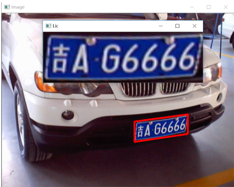
This distortion is caused by the projection caused by the camera not perpendicular to the license plate, so it can be corrected by CV2. Warpprective().

# Transformation matrix
mat = cv2.getPerspectiveTransform(point_set_0, point_set_1)
# Projection transformation
lic = cv2.warpPerspective(img, mat, (440, 140))

# Created by Dan Cheng senior: Q746876041
import cv2
import numpy as np

# Pretreatment
def imgProcess(path):
    img = cv2.imread(path)
    # Uniform size
    img = cv2.resize(img, (640,480))
    # Gaussian blur
    img_Gas = cv2.GaussianBlur(img,(5,5),0)
    # RGB channel separation
    img_B = cv2.split(img_Gas)[0]
    img_G = cv2.split(img_Gas)[1]
    img_R = cv2.split(img_Gas)[2]
    # Read gray image and HSV space image
    img_gray = cv2.cvtColor(img_Gas, cv2.COLOR_BGR2GRAY)
    img_HSV = cv2.cvtColor(img_Gas, cv2.COLOR_BGR2HSV)
    return img, img_Gas, img_B, img_G, img_R, img_gray, img_HSV

# Preliminary identification
def preIdentification(img_gray, img_HSV, img_B, img_R):
    for i in range(480):
        for j in range(640):
            # Ordinary blue license plate, while excluding the interference of transparent reflective materials
            if ((img_HSV[:, :, 0][i, j]-115)**2 < 15**2) and (img_B[i, j] > 70) and (img_R[i, j] < 40):
                img_gray[i, j] = 255
            else:
                img_gray[i, j] = 0
    # Define core
    kernel_small = np.ones((3, 3))
    kernel_big = np.ones((7, 7))

    img_gray = cv2.GaussianBlur(img_gray, (5, 5), 0) # Gaussian smoothing
    img_di = cv2.dilate(img_gray, kernel_small, iterations=5) # Corrosion for 5 times
    img_close = cv2.morphologyEx(img_di, cv2.MORPH_CLOSE, kernel_big) # Closed operation
    img_close = cv2.GaussianBlur(img_close, (5, 5), 0) # Gaussian smoothing
    _, img_bin = cv2.threshold(img_close, 100, 255, cv2.THRESH_BINARY) # Binarization
    return img_bin

# location
def fixPosition(img, img_bin):
    # Detect all outer contours, leaving only four vertices of the rectangle
    contours, _ = cv2.findContours(img_bin, cv2.RETR_LIST, cv2.CHAIN_APPROX_SIMPLE)
    #Shape and size screening verification
    det_x_max = 0
    det_y_max = 0
    num = 0
    for i in range(len(contours)):
        x_min = np.min(contours[i][ :, :, 0])
        x_max = np.max(contours[i][ :, :, 0])
        y_min = np.min(contours[i][ :, :, 1])
        y_max = np.max(contours[i][ :, :, 1])
        det_x = x_max - x_min
        det_y = y_max - y_min
        if (det_x / det_y > 1.8) and (det_x > det_x_max ) and (det_y > det_y_max ):
            det_y_max = det_y
            det_x_max = det_x
            num = i
    # Get the contour point set of the most suspicious area
    points = np.array(contours[num][:, 0])
    return points


#img_lic_canny = cv2.Canny(img_lic_bin, 100, 200)


def findVertices(points):
    # Obtain the minimum circumscribed matrix, center point coordinates, width, height and rotation angle
    rect = cv2.minAreaRect(points)
    # Gets the four vertices of a rectangle, floating point
    box = cv2.boxPoints(rect)
    # Rounding
    box = np.int0(box)
    # Get four vertex coordinates
    left_point_x = np.min(box[:, 0])
    right_point_x = np.max(box[:, 0])
    top_point_y = np.min(box[:, 1])
    bottom_point_y = np.max(box[:, 1])

    left_point_y = box[:, 1][np.where(box[:, 0] == left_point_x)][0]
    right_point_y = box[:, 1][np.where(box[:, 0] == right_point_x)][0]
    top_point_x = box[:, 0][np.where(box[:, 1] == top_point_y)][0]
    bottom_point_x = box[:, 0][np.where(box[:, 1] == bottom_point_y)][0]
    # Up, down, left and right coordinates
    vertices = np.array([[top_point_x, top_point_y], [bottom_point_x, bottom_point_y], [left_point_x, left_point_y], [right_point_x, right_point_y]])
    return vertices, rect

def tiltCorrection(vertices, rect):
    # Distortion condition 1
    if rect[2] > -45:
        new_right_point_x = vertices[0, 0]
        new_right_point_y = int(vertices[1, 1] - (vertices[0, 0]- vertices[1, 0]) / (vertices[3, 0] - vertices[1, 0]) * (vertices[1, 1] - vertices[3, 1]))
        new_left_point_x = vertices[1, 0]
        new_left_point_y = int(vertices[0, 1] + (vertices[0, 0] - vertices[1, 0]) / (vertices[0, 0] - vertices[2, 0]) * (vertices[2, 1] - vertices[0, 1]))
        # Corrected four vertex coordinates
        point_set_1 = np.float32([[440, 0],[0, 0],[0, 140],[440, 140]])
    # Distortion condition 2
    elif rect[2] < -45:
        new_right_point_x = vertices[1, 0]
        new_right_point_y = int(vertices[0, 1] + (vertices[1, 0] - vertices[0, 0]) / (vertices[3, 0] - vertices[0, 0]) * (vertices[3, 1] - vertices[0, 1]))
        new_left_point_x = vertices[0, 0]
        new_left_point_y = int(vertices[1, 1] - (vertices[1, 0] - vertices[0, 0]) / (vertices[1, 0] - vertices[2, 0]) * (vertices[1, 1] - vertices[2, 1]))
        # Corrected four vertex coordinates
        point_set_1 = np.float32([[0, 0],[0, 140],[440, 140],[440, 0]])

    # Coordinates of four vertices of parallelogram before correction
    new_box = np.array([(vertices[0, 0], vertices[0, 1]), (new_left_point_x, new_left_point_y), (vertices[1, 0], vertices[1, 1]), (new_right_point_x, new_right_point_y)])
    point_set_0 = np.float32(new_box)
    return point_set_0, point_set_1, new_box

def transform(img, point_set_0, point_set_1):
    # Transformation matrix
    mat = cv2.getPerspectiveTransform(point_set_0, point_set_1)
    # Projection transformation
    lic = cv2.warpPerspective(img, mat, (440, 140))
    return lic

def main():
    path = 'F:\\Python\\license_plate\\test\\9.jpg'
    # Image preprocessing
    img, img_Gas, img_B, img_G, img_R, img_gray, img_HSV = imgProcess(path)
    # Preliminary identification
    img_bin  = preIdentification(img_gray, img_HSV, img_B, img_R)
    points = fixPosition(img, img_bin)
    vertices, rect = findVertices(points)
    point_set_0, point_set_1, new_box = tiltCorrection(vertices, rect)
    img_draw = cv2.drawContours(img.copy(), [new_box], -1, (0,0,255), 3)
    lic = transform(img, point_set_0, point_set_1)
    # The license plate is framed on the original drawing
    cv2.namedWindow("Image")
    cv2.imshow("Image", img_draw)
    # Binary image
    cv2.namedWindow("Image_Bin")
    cv2.imshow("Image_Bin", img_bin)
    # Display corrected license plate
    cv2.namedWindow("Lic")
    cv2.imshow("Lic", lic)
    # Pause, close window
    cv2.waitKey(0)
    cv2.destroyAllWindows()

if __name__ == '__main__':
    main()

7 finally - design help

Bi design help, problem opening guidance, technical solutions
🇶746876041