1, Multilayer perceptron model based on BP algorithm
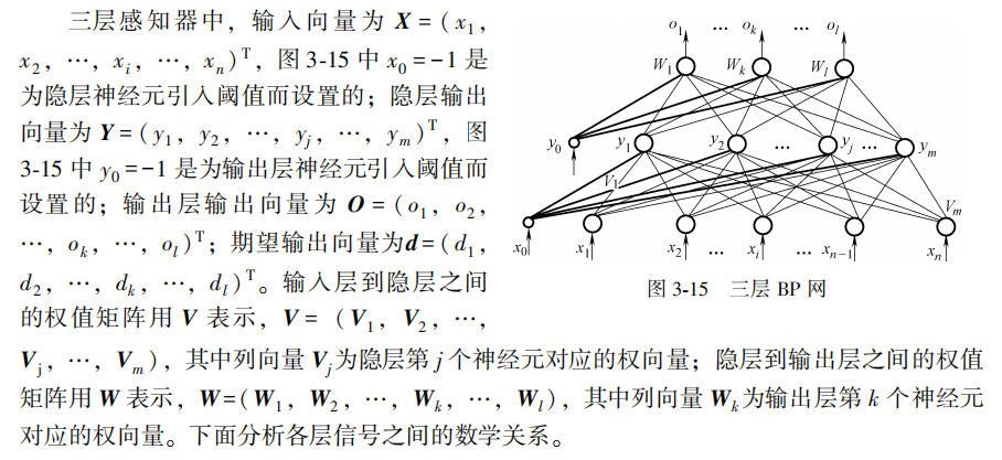
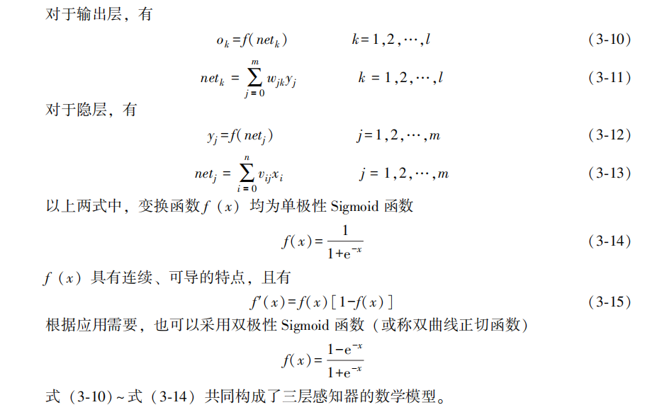
The multilayer perceptron using BP algorithm is the most widely used neural network so far. In the application of multilayer perceptron, the single hidden layer network shown in Figure 3-15 is the most common. In general, it is customary to call a single hidden layer feedforward network a three-layer perceptron. The so-called three layers include input layer, hidden layer and output layer.
The final result of the algorithm adopts the gradient descent method, and the specific detailed process is omitted here!
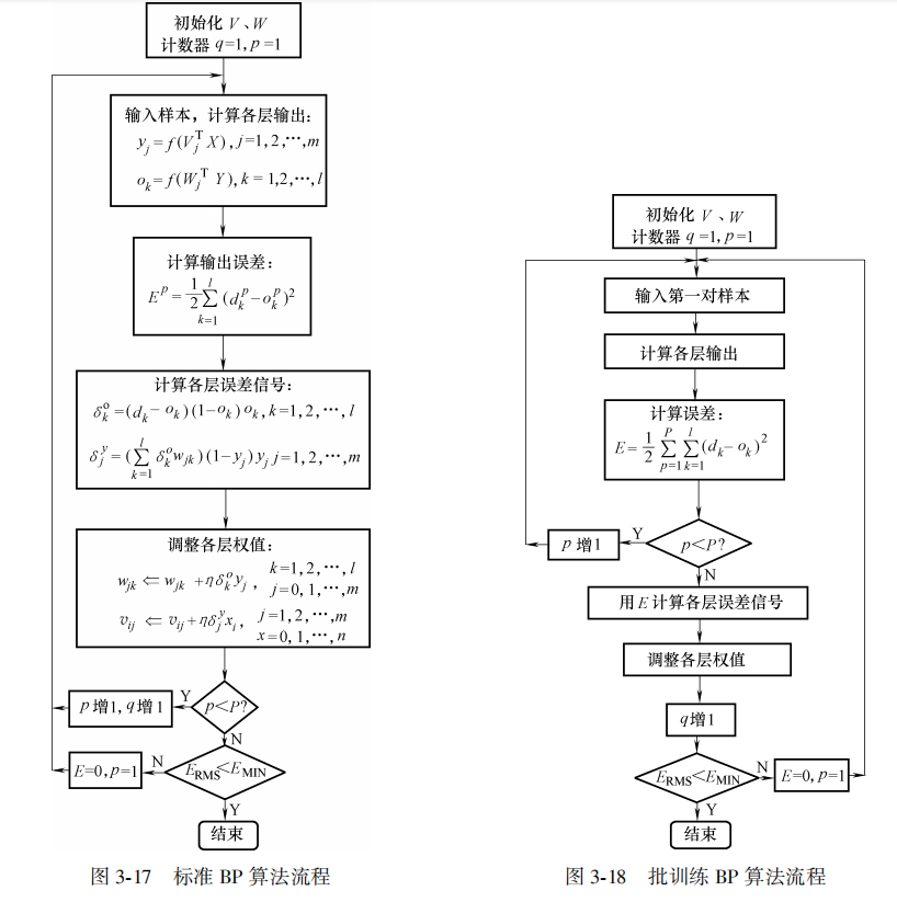
2, Program implementation flow of BP algorithm
3, Improvement of standard BP algorithm -- adding momentum term
When adjusting the weights, the standard BP algorithm only adjusts according to the gradient descent direction of the error at time t, without considering the gradient direction before time t, which often makes the training process oscillate and converge slowly. In order to improve the training speed of the network, a momentum term can be added to the weight adjustment formula. If W represents the weight matrix of a layer and X represents the input vector of a layer, the expression of the weight adjustment vector containing momentum term is
It can be seen that increasing the momentum term means taking out part of the previous weight adjustment and adding it to the current weight adjustment, α It is called the momentum coefficient, which generally has a ∈ (0,1). The momentum term reflects the adjustment experience accumulated before and plays a damping role in the adjustment of time t. When the error surface fluctuates suddenly, the oscillation trend can be reduced and the training speed can be improved. At present, the momentum term is added to the BP algorithm, so that the BP algorithm with momentum term has become a new standard algorithm.
4, Implementing BP neural network and its learning algorithm with Python
Here, in order to use the algorithm, a brief example is given (no normalization or standardization is required)
Enter X=-1:0.1:1;
Output D =.... (see the data in the code for details)
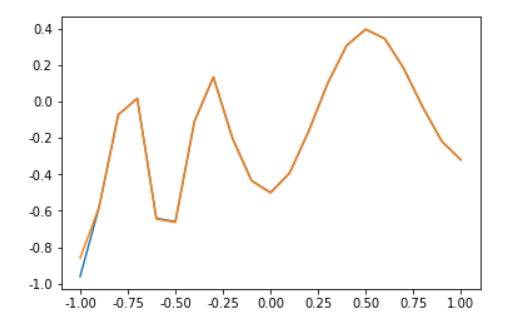
In order to view the results, we draw the results as graphs, as follows:
The yellow line and blue line represent the output and input after training
5, The procedure is as follows:
# -*- coding: utf-8 -*-
import math
import string
import matplotlib as mpl
############################################Call library (modify according to your own programming)
import numpy.matlib
import numpy as np
np.seterr(divide='ignore',invalid='ignore')
import matplotlib.pyplot as plt
from matplotlib import font_manager
import pandas as pd
import random

#Generating random numbers in interval [a,b]
def random_number(a,b):
    return (b-a)*random.random()+a

#Generate a matrix with the size of m*n, and set the default zero matrix
def makematrix(m, n, fill=0.0):
    a = []
    for i in range(m):
        a.append([fill]*n)
    return np.array(a)

#Function sigmoid(), both functions can be used as activation functions
def sigmoid(x):
    #return np.tanh(x)
    return (1-np.exp(-1*x))/(1+np.exp(-1*x))
#Functions derived from sigmoid
def derived_sigmoid(x):
    return 1-(np.tanh(x))**2
    #return (2*np.exp((-1)*x)/((1+np.exp(-1*x)**2)))

#Construct three-layer BP network architecture
class BPNN:
    def __init__(self, num_in, num_hidden, num_out):
        #Number of nodes in input layer, hidden layer and output layer
        self.num_in = num_in + 1  #Add an offset node
        self.num_hidden = num_hidden + 1   #Add an offset node
        self.num_out = num_out

        #Activate all nodes (vectors) of the neural network
        self.active_in = np.array([-1.0]*self.num_in)
        self.active_hidden = np.array([-1.0]*self.num_hidden)
        self.active_out = np.array([1.0]*self.num_out)

        #Create weight matrix
        self.wight_in = makematrix(self.num_in, self.num_hidden)
        self.wight_out = makematrix(self.num_hidden, self.num_out)

        #Assign initial value to weight matrix
        for i in range(self.num_in):
            for j in range(self.num_hidden):
                self.wight_in[i][j] = random_number(0.1, 0.1)
        for i in range(self.num_hidden):
            for j in range(self.num_out):
                self.wight_out[i][j] = random_number(0.1, 0.1)
        #deviation
        for j in range(self.num_hidden):
            self.wight_in[0][j] = 0.1
        for j in range(self.num_out):
            self.wight_in[0][j] = 0.1


        #Finally, the momentum factor (matrix) is established
        self.ci = makematrix(self.num_in, self.num_hidden)
        self.co = makematrix(self.num_hidden, self.num_out)


    #Signal forward propagation
    def update(self, inputs):
        if len(inputs) != self.num_in-1:
            raise ValueError('Inconsistent with the number of input layer nodes')
        #Data input layer
        self.active_in[1:self.num_in]=inputs

        #Data processing in hidden layer
        self.sum_hidden=np.dot(self.wight_in.T,self.active_in.reshape(-1,1)) #Dot multiplication
        self.active_hidden=sigmoid(self.sum_hidden)   #active_hidden [] is stored after processing the input data as the input data of the output layer
        self.active_hidden[0]=-1

        #Data processing in the output layer
        self.sum_out=np.dot(self.wight_out.T,self.active_hidden) #Dot multiplication
        self.active_out = sigmoid(self.sum_out)   #Same as above
        return self.active_out


    #Error back propagation
    def errorbackpropagate(self, targets, lr,m):   #lr is the learning rate
        if self.num_out==1:
            targets=[targets]
        if len(targets) != self.num_out:
            raise ValueError('Inconsistent with the number of output layer nodes!')
        #error
        error=(1/2)*np.dot((targets.reshape(-1,1)-self.active_out).T,(targets.reshape(-1,1)-self.active_out))

        #Output error signal
        self.error_out=(targets.reshape(-1,1)-self.active_out)*derived_sigmoid(self.sum_out)
        #Hidden layer error signal
        #self.error_hidden=np.dot(self.wight_out.reshape(-1,1),self.error_out.reshape(-1,1))*self.active_hidden*(1-self.active_hidden)
        self.error_hidden=np.dot(self.wight_out,self.error_out)*derived_sigmoid(self.sum_hidden)

        #Update weight
        #hide
        self.wight_out=self.wight_out+lr*np.dot(self.error_out,self.active_hidden.reshape(1,-1)).T+m*self.co
        self.co=lr*np.dot(self.error_out,self.active_hidden.reshape(1,-1)).T
        #input
        self.wight_in=self.wight_in+lr*np.dot(self.error_hidden,self.active_in.reshape(1,-1)).T+m*self.ci
        self.ci=lr*np.dot(self.error_hidden,self.active_in.reshape(1,-1)).T
        return error

    #test
    def test(self, patterns):
        for i in patterns:
            print(i[0:self.num_in-1], '->', self.update(i[0:self.num_in-1]))
        return self.update(i[0:self.num_in-1])

    #Weight
    def weights(self):
        print("Enter layer weights")
        print(self.wight_in)
        print("Output layer weight")
        print(self.wight_out)

    def train(self, pattern, itera=100, lr = 0.2, m=0.1):
        for i in range(itera):
            error = 0.0
            for j in pattern:
                inputs = j[0:self.num_in-1]
                targets = j[self.num_in-1:]
                self.update(inputs)
                error = error+self.errorbackpropagate(targets, lr,m)
            if i % 10 == 0:
                print('########################error %-.5f######################Iteration% d '% (error,i))

#example
X=list(np.arange(-1,1.1,0.1))
D=[-0.96, -0.577, -0.0729, 0.017, -0.641, -0.66, -0.11, 0.1336, -0.201, -0.434, -0.5, -0.393, -0.1647, 0.0988, 0.3072, 0.396, 0.3449, 0.1816, -0.0312, -0.2183, -0.3201]
A=X+D
patt=np.array([A]*2)
    #Create neural network, 21 input nodes, 21 hidden layer nodes and 1 output layer node
n = BPNN(21, 21, 21)
    #Training neural network
n.train(patt)
    #Test neural network
d=n.test(patt)
    #View weight value
n.weights()

plt.plot(X,D)
plt.plot(X,d)
plt.show()
Source: Xiaoling Blog - Good Times is not a good Blog
[1] Han Liqun, artificial neural network theory and application [M] Beijing: China Machine Press, 2016


