Anomaly detection -- from classical algorithms to deep learning 14. RRCF based anomaly detection for stream data

Anomaly detection: from classical algorithms to deep learning

relevant:

14. RRCF based anomaly detection for stream data

2016 Robust random cut forest based anomaly detection on streams
Thesis download and source address github
The paper was published in ccml (International Conference on Machine Learning) CCF A
Implementation of RRCF Download address
For the translation part, please go to my personal blog: smileyan.cn

14.1 brief overview of the paper

14.1.1 core ideas and methods

Random forest (RF) is a bagging algorithm. RRCF (Robust Random Cut Forest) mentioned in this paper is improved on the basis of RF to achieve the effect of "robustness". Therefore, the core idea of this paper is to improve RF into RRCF, define and prove some properties of RRCF, and experiment to prove the effect of RRCF.

Therefore, the whole paper should include the following aspects:

What is RRCF?
Where is the improvement of RRCF relative to RF and how?
How RRCF is applied to anomaly detection of stream data (i.e. time series data).

Because there are many definitions, we will look down one by one.

14.1.2 RRCF generation process

First, learn about the RF generation process, which is very helpful to continue to understand RRCF.

The goal of the integration method is to combine the prediction of multiple basic estimators with a given learning algorithm to improve the generality / robustness of a single classifier. There are two integration methods: Boosting and bagging. Random forest is a typical representative of bagging.

The generation process of random forest can be parallel, that is to say,

The generation of each tree is irrelevant;
The sampling of the corresponding data generated by each tree is also irrelevant (random sampling with return)
The status of each tree is equal, which is very different from boosting thought.

Then, it is specific to the generation of each tree, which is no different from the construction steps of decision tree. The generation process of the decision tree is easy to understand. It is basically understood by referring to the job search process. First, the salary can not be less than how much, which is divided into two categories, and then the year-end salary can not be less than how much, which continues to be divided into two categories, etc.

Next, focus on the generation process of RRCF, that is, the definition 1 in the paper:

Definition 1 for a point set S S S. A robust random partition tree is generated as follows:

Select a and ℓ i ∑ j ℓ j \frac{\ell_i}{\sum_j \ell_j} Σ j ℓ j ℓ i proportional random dimension, where ℓ i = m a x x ∈ S x i − m i n x ∈ S x i \ell_i = max_{x\in S}x_i-min_{x\in S}x_i ℓi=maxx∈Sxi−minx∈Sxi.
Choose one X i ∼ U n i f o r m [ m i n x ∈ S x i , m a x x ∈ S x i ] X_i \sim Uniform[min_{x\in S} x_i, max_{x\in S}x_i] Xi ∈ Uniform[minx ∈ S Xi, maxx ∈ S Xi] is the uniform distribution from minimum to maximum.
set up S 1 = { x ∣ x ∈ S , x i ≤ X i } S_1=\{x|x\in S,x_i\le X_i\} S1={x∣x∈S,xi≤Xi} ， S 2 = S S 1 S_2=S\ \text{\\}\ S_1 S2=S S1 ・ and based on S 1 S_1 S1} and S 2 S_2 Recursion of S2.

Related theorem 1

Theorem 1 (Theorem 1)

Consider the algorithm in definition 1. Let the weight of the nodes in the tree be the sum of the corresponding dimensions ∑ i ℓ i \sum_i \ell_i ∑iℓi. Given two points u , v ∈ S u,v\in S u. V ∈ S, will u u u and v v The tree distance between v is defined as u , v u, v u. The weight of the minimum common ancestor of V. Then, the minimum distance between trees is Manhattan distance L 1 ( u , v ) L_1(u,v) L1 (u,v), the maximum distance is O ( d log ⁡ ∣ S ∣ L 1 ( u , v ) ) ∗ L 1 ( u , v ) O(d\log \frac{|S|}{L_1(u,v)})*L_1(u,v) O(dlogL1(u,v)∣S∣)∗L1(u,v).

14.1.3 RRCF segmentation process

Theorem 2 (theorem 2)

Given a basis T ( S ) \mathcal{T}(S) T(S) generates a tree if we delete it that contains outliers x x x ， and its parent node (adjust the grandparent point accordingly, as shown in Figure 2), the generated tree T ′ T' Probability and of T ' T ( S − { x } ) \mathcal{T}(S-\{x\}) The probability generated in T(S − {x}) is the same. Similarly, we can generate a tree T ′ ′ T'' T 'is like from T ( S ∪ { x } ) T(S\ \cup \{x\}) T(S ∪ {x}) like random sampling, when the maximum depth is T T When T, its generation time complexity is O ( d ) O(d) O(d), which is usually ∣ T ∣ |T| ∣ T ∣ sublinear.

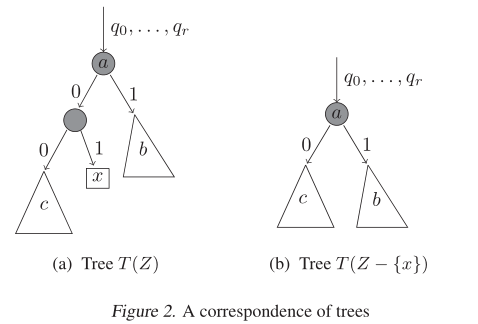
This is understandable. What's left after cutting c c c represents the entire parent node before it, and the probability will not change naturally.

The following theorems 3, 4 and 5 can be looked at a little, and some performance considerations.

14.1.4 defining exceptions

Firstly, the paper gives an example of someone wearing a hat to change color. To be honest, this example is not very good.

Definition 2

Will point x x The bit displacement or displacement of x is defined as the increase in the model complexity of all other points, that is, for the set Z Z Z. To capture x x Externalities (outliers) of x, definition
D I S P ( x , Z ) = ∑ T , y ∈ Z − { x } P r [ T ] ( f ( y , Z , T ) − f ( y , Z − { x } , T ′ ) ) DISP(x, Z)=\sum_{T, y\in Z-\{x\}} \mathbb{P}r[T](f(y,Z,T)-f(y,Z-\{x\},T')) DISP(x,Z)=T,y∈Z−{x}∑Pr[T](f(y,Z,T)−f(y,Z−{x},T′))
among T ′ = T ( Z − { x } ) T'=T(Z-\{x\}) T′=T(Z−{x}) .

1The converse is not true, this is a many-to-one mapping.

Conversely, this is a many to one mapping.

14.1.5 flow based forest maintenance

Insertion: given from R R C F ( S ) RRCF(S) Samples from RRCF(S) distribution T T T and point p ∉ S p \not \in S p ∈ S, from R R C F ( S ∪ { p } ) RRCF(S\cup \{p\}) Samples are extracted from RRCF(S ∪ {p}) distribution T ′ T' T′.

Detection: given from R R C F ( S ) RRCF(S) Samples from RRCF(S) distribution T T T and point p ∈ S p \in S p ∈ S, from R R C F ( S ∪ { p } ) RRCF(S\cup \{p\}) Samples are extracted from RRCF(S ∪ {p}) distribution T ′ T' T′. We need to make the following simple observations.

Observation 1 if and only if the axis parallel cut can be used to separate the minimum axis aligned bounding box B ( S ) B(S) B(S) and p p p, you can use the axis parallel cut to separate the point set S S S and p p p .

The next lemma provides structural properties about RRCF trees. We are interested in incremental updates, making as few changes as possible to a set of trees. Please note that given a specific tree, we have two detailed situations: (i) the new points to be deleted (inserted separately) are not separated by the first cut, and (ii) the new points to be deleted (inserted separately) are separated by the first cut. Lemma 3 solves these problems for a set of trees (not just a tree) satisfying (i) and (ii) respectively

Lemma 3 (Lemma 3)

Given point p p p and a set of points S S S. Its axis is parallel to the minimum bounding box B ( S ) B(S) B(S), so that p ∉ B p\not \in B p∈B:

For any dimension i i i. Select dimensions using the weighted isolated forest algorithm i i The probability of splitting axis parallel cutting in i is exactly the same as the conditional probability of selecting splitting axis parallel cutting S ∪ { p } S\cup \{p\} S ∪ {p}, provided that p p p and S S All points of S are isolated.
given R R C F ( S ) RRCF(S) Random tree of RRCF(S) S ∪ { p } S\cup \{p\} S ∪ {p}, provided that the first cut will p p p and S S All points of S are isolated, and the rest of the tree is R R C F ( S ) RRCF(S) Random tree in RRCF(S).

Refer to for more information smileyan.cn

14.2 hands on experiment

The corresponding algorithm source code is in github.com It has been implemented, and there are even relatively complete document examples https://klabum.github.io/rrcf/ , you might as well go and experience it.

Note that there is also a brief introduction paper on the implementation of the algorithm Go and check .

14.2.1 environmental installation

Ensure the environment of Python 3, and then enter the command:

$ pip install rrcf

Ready to install.

RRCF dependencies include:

numpy (>= 1.15)

Examples provided by RRCF include:

pandas (>= 0.23)
scipy (>= 1.2)
scikit-learn (>= 0.20)
matplotlib (>= 3.0)

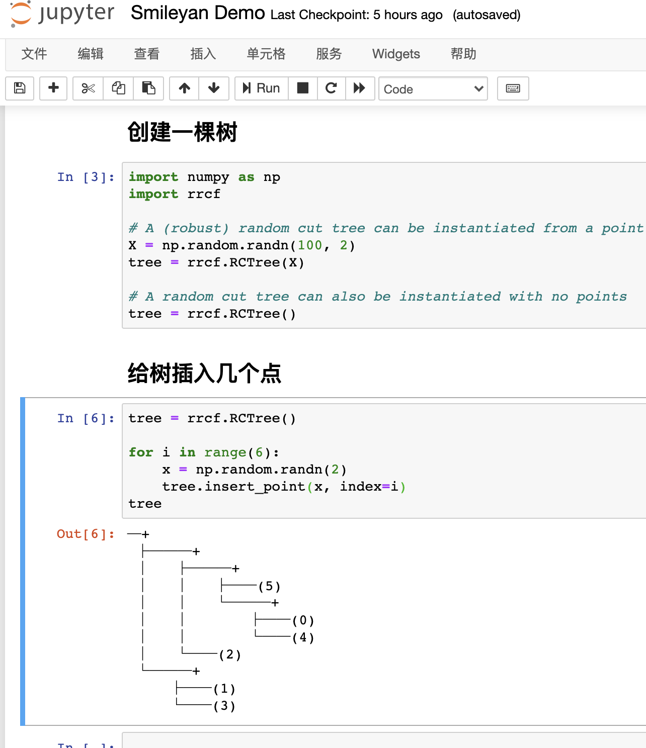
14.2.2 first example

Create a tree,

import numpy as np
import rrcf

# A (robust) random cut tree can be instantiated from a point set (n x d)
X = np.random.randn(100, 2)
tree = rrcf.RCTree(X)

# A random cut tree can also be instantiated with no points
tree = rrcf.RCTree()

Insert several points into the tree:

tree = rrcf.RCTree()

for i in range(6):
    x = np.random.randn(2)
    tree.insert_point(x, index=i)
tree

The following effects can be seen at this time:

Delete node 2,

tree.forget_point(2)

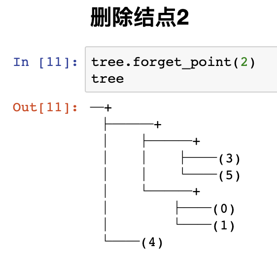
Note that this has nothing to do with exception detection, but indicates that RRCF has these functions.

14.2.3 RRCF is used for anomaly detection

As mentioned earlier, when a point is inserted, which greatly increases the complexity of the model, it is very likely to be an outlier. Here is an example (officially provided).

# Seed tree with zero-mean, normally distributed data
X = np.random.randn(100,2)
tree = rrcf.RCTree(X)

# Generate an inlier and outlier point
inlier = np.array([0, 0])
outlier = np.array([4, 4])

# Insert into tree
tree.insert_point(inlier, index='inlier')
tree.insert_point(outlier, index='outlier')

The code starts with normally distributed data as a training set, which is used to generate numbers 🌲.

Then insert two points (0, 0) and (4,4). It is obvious that (4,4) does not conform to the normal distribution.

Finally, these two points are inserted with an index to facilitate searching.

Then look at the complexity of inserting these two points into the model.

tree.codisp('inlier')

tree.codisp('outlier')

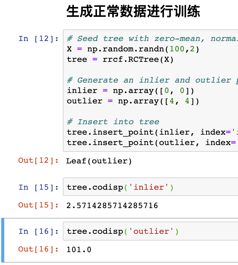
Note that since the data is generated randomly, it is normal for the results to be inconsistent, but the output of normal data will be much smaller than that of abnormal data.

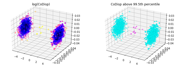
14.2.4 RRCF is used for batch anomaly detection

The same data is made, but this time it is tested on a large scale in the form of batches.

import numpy as np
import pandas as pd
import rrcf

# Set sample parameters
np.random.seed(0)
n = 2010
d = 3

# Generate data
X = np.zeros((n, d))
X[:1000,0] = 5
X[1000:2000,0] = -5
X += 0.01*np.random.randn(*X.shape)

# Set forest parameters
num_trees = 100
tree_size = 256
sample_size_range = (n // tree_size, tree_size)

# Construct forest
forest = []
while len(forest) < num_trees:
    # Select random subsets of points uniformly
    ixs = np.random.choice(n, size=sample_size_range,
                           replace=False)
    # Add sampled trees to forest
    trees = [rrcf.RCTree(X[ix], index_labels=ix)
             for ix in ixs]
    forest.extend(trees)

# Compute average CoDisp
avg_codisp = pd.Series(0.0, index=np.arange(n))
index = np.zeros(n)
for tree in forest:
    codisp = pd.Series({leaf : tree.codisp(leaf)
                       for leaf in tree.leaves})
    avg_codisp[codisp.index] += codisp
    np.add.at(index, codisp.index.values, 1)
avg_codisp /= index

After the calculation, the following code is shown:

from mpl_toolkits.mplot3d import Axes3D
import matplotlib.pyplot as plt
from matplotlib import colors

threshold = avg_codisp.nlargest(n=10).min()

fig = plt.figure(figsize=(12,4.5))
ax = fig.add_subplot(121, projection='3d')
sc = ax.scatter(X[:,0], X[:,1], X[:,2],
                c=np.log(avg_codisp.sort_index().values),
                cmap='gnuplot2')
plt.title('log(CoDisp)')
ax = fig.add_subplot(122, projection='3d')
sc = ax.scatter(X[:,0], X[:,1], X[:,2],
                linewidths=0.1, edgecolors='k',
                c=(avg_codisp >= threshold).astype(float),
                cmap='cool')
plt.title('CoDisp above 99.5th percentile')

The effect picture is:

14.2.5 RRCF is used for stream data anomaly detection

First, generate data and detect exceptions

import numpy as np
import rrcf

# Generate data
n = 730
A = 50
center = 100
phi = 30
T = 2*np.pi/100
t = np.arange(n)
sin = A*np.sin(T*t-phi*T) + center
sin[235:255] = 80

# Set tree parameters
num_trees = 40
shingle_size = 4
tree_size = 256

# Create a forest of empty trees
forest = []
for _ in range(num_trees):
    tree = rrcf.RCTree()
    forest.append(tree)
    
# Use the "shingle" generator to create rolling window
points = rrcf.shingle(sin, size=shingle_size)

# Create a dict to store anomaly score of each point
avg_codisp = {}

# For each shingle...
for index, point in enumerate(points):
    # For each tree in the forest...
    for tree in forest:
        # If tree is above permitted size, drop the oldest point (FIFO)
        if len(tree.leaves) > tree_size:
            tree.forget_point(index - tree_size)
        # Insert the new point into the tree
        tree.insert_point(point, index=index)
        # Compute codisp on the new point and take the average among all trees
        if not index in avg_codisp:
            avg_codisp[index] = 0
        avg_codisp[index] += tree.codisp(index) / num_trees

Display of calculation results

import pandas as pd
import matplotlib.pyplot as plt
import seaborn as sns

fig, ax1 = plt.subplots(figsize=(10, 5))

color = 'tab:red'
ax1.set_ylabel('Data', color=color, size=14)
ax1.plot(sin, color=color)
ax1.tick_params(axis='y', labelcolor=color, labelsize=12)
ax1.set_ylim(0,160)
ax2 = ax1.twinx()
color = 'tab:blue'
ax2.set_ylabel('CoDisp', color=color, size=14)
ax2.plot(pd.Series(avg_codisp).sort_index(), color=color)
ax2.tick_params(axis='y', labelcolor=color, labelsize=12)
ax2.grid('off')
ax2.set_ylim(0, 160)
plt.title('Sine wave with injected anomaly (red) and anomaly score (blue)', size=14)

14.3 summary

Anomaly detection has a long way to go. RRCF can be used as a representative of classical machine learning algorithms for comparative experiments. It can be said that it is a relatively advanced representative.

The expression of the paper is a little strange, but the general meaning should be understandable. If you have any questions, please leave a message below and let's discuss it together.

Smileyan
2021.11/28 18:09

[1] Paper address
[2] Source address

Posted by mrblom on Sun, 28 Nov 2021 06:46:26 -0800

Programmer Group