Project code
reference resources Know and never forget the original heart
1. Implementation of SVM
The previous section is mainly about the acquisition of Chinese word segmentation and word vector expression. However, each article contains a different number of words, so this paper represents the document by calculating the average word vector, that is, the vectors containing all words in the article are added and averaged, so that a vector pointing to the article information with the same dimension as the word vector can be obtained.
import numpy as np
import pandas as pd
import gensim
# num_feature represents the text word size

def average_word_vectors(words,model,vocabulary,num_features):
    feature_vector=np.zeros((num_features,),dtype='float64')
    nwords=0
    for word in words:
        if word in vocabulary:
            nwords+=1
            feature_vector=np.add(feature_vector,model.key_to_index[word])
    if nwords:
        # Because of averaging
        feature_vector=np.divide(feature_vector,nwords)
    return feature_vector

def average_word_vectorized(corpus,model,num_features):
    vocabulary=set(model.index_to_key)
    features=[average_word_vectors(tokenized_sentence,model,vocabulary,num_features) for tokenized_sentence in corpus]
    return np.array(features)

def get_word_vectors(data):
    words_art=[]
    for i in range(len(data)):
        words_art.append(eval(data.loc[i]))
    return average_word_vectorized(words_art,model=w2v_model,num_features=300)
After calculating the average vector, the following applies to the word segmentation list saved in the form of article in advance.
w2v_model=gensim.models.KeyedVectors.load_word2vec_format('data/word2vec_model.txt',binary=False)
train=pd.read_csv('data/article_features_train.csv')
test=pd.read_csv('data/article_features_test.csv')
x_train=get_word_vectors(train.Words)
y_train=train.label
x_test=get_word_vectors(test.Words)
y_test=test.label
Then the grid search algorithm GridSearchCV is used to find f1_macro's highest model
# Find F1 using GSCV_ Macro's highest model
from sklearn import svm
from sklearn.model_selection import GridSearchCV
from sklearn.metrics import f1_score
clf=svm.SVC()
grid_values={'gamma':[0.001, 0.01, 0.05, 0.1, 1, 10],
             'C':[0.01, 0.1, 1, 10, 100]}

grid_clf=GridSearchCV(clf,param_grid=grid_values,scoring='f1_macro')
grid_clf.fit(x_train,y_train)
y_grid_pred=grid_clf.predict(x_test)

print('Test set F1: ', f1_score(y_test,y_grid_pred,average='macro'))
print('Grid best parameter (max. f1): ', grid_clf.best_params_)
print('Grid best score (accuracy): ', grid_clf.best_score_)
The output is as follows:
- Test set F1: 0.35209688361418695
- Grid best parameter (max. f1): {'C': 100, 'gamma': 1}
- Grid best score (accuracy): 0.3681357073595844
After setting these parameters, retrain and save the model
import seaborn as sns
import matplotlib.pyplot as plt
import matplotlib
cm=confusion_matrix(y_test,y_pred)

# Drawing the conflict matrix
print('Confusion Matrix')
category_labels=['Space ','Computer ','Art ', 'Environment ', 'Agriculture ', 'Economy ','Politics ','Sports ','History ']
cm_normalised=cm.astype('float')/cm.sum(axis=1)[:,np.newaxis]
sns.set(font_scale=1.5)
fig,ax=plt.subplots(figsize=(10,10))
ax=sns.heatmap(cm_normalised,annot=True,linewidths=1,square=False,
               cmap='Greens',yticklabels=category_labels,xticklabels=category_labels,
               vmin=0,vmax=np.max(cm_normalised),fmt='.2f',annot_kws={'size':20})
ax.set(xlabel='Predicted label',ylabel='True label')
2. TextCNN implementation
In addition to simple SVM classifier, neural network is also tried here. Although CNN is widely used in image processing, it also has its place in text processing. Next, we will build a TextCNN model to implement the classification task. First, we need to preprocess the word2vec model. The Embedding layer in TextCNN requires us to convert word segmentation into index, so we convert the words in the model into a dictionary and save it in [word: index] for future processing.
# Import w2v model and preprocess
def w2v_model_preprocessing():
    w2v_model=gensim.models.KeyedVectors.load_word2vec_format('data/word2vec_model.txt',binary=False)

    # Initialize the [word:index] dictionary
    word2idx={'_PAD':0}
    vocab_list=[(k,w2v_model.key_to_index[k]) for k,v in w2v_model.key_to_index.items()]
    # Store an array of all vectors in all w2v, including one more bit, and all word vectors are 0, which is used for padding
    embeddings_matrix=np.zeros((len(w2v_model.key_to_index.items())+1,w2v_model.vector_size))
    # Fill dictionary and matrix
    for i in range(len(vocab_list)):
        word=vocab_list[i][0]
        word2idx[word]=i+1
        embeddings_matrix[i+1]=vocab_list[i][1]
    return w2v_model,word2idx,embeddings_matrix

w2v_model,word2idx,embeddings_matrix=w2v_model_preprocessing()
Similarly, we still face the same problem as when building SVM: how to deal with the difference of article length. Here, we consider the solution of truncation, that is, specify a length in advance. If it is insufficient, fill in zero later, and if it exceeds, round off all the contents later, so as to achieve the purpose of consistent length.
from tensorflow.keras.preprocessing.sequence import pad_sequences

def get_words(data):
    words_art=[]
    for i in range(len(data)):
        words_art.append(eval(data.loc[i]))
    return words_art

#The obtained Chinese word segmentation is transformed with the generated dictionary. Get the word segmentation index array with the same length as maxlen. If it exceeds, it will be truncated, and if it is insufficient, it will be followed by zero
#Text is text, word_index is the dictionary and maxlen is the length of the array to be saved
def get_words_index(text,word_index,maxlen):
    texts=get_words(text)
    data=[]
    for sentence in texts:
        new_txt=[]
        for word in sentence:
            try:
                # Convert the participle in the sentence to index
                new_txt.append(word_index[word])
            except:
                new_txt.append(0)
        data.append(new_txt)
    # Use kears' built-in function padding to align sentences
    texts=pad_sequences(data,maxlen=maxlen,padding='post')
    return texts
Next, we read the file and convert the word segmentation of the article into the form of index. The length of each article in the training set, that is, the distribution of the number of words contained, is shown in the figure below.
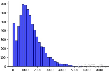
In this practice, we set the truncation length to 1000.
from tensorflow.keras.utils import to_categorical
from sklearn.model_selection import train_test_split

MAX_LENGTH=1000
# Load training and test sets
train=pd.read_csv('data/article_features_train.csv')
test=pd.read_csv('data/article_features_test.csv')

# Training set data preprocessing
x_train=get_words_index(train.Words,word2idx,MAX_LENGTH)
y_train=train.label
y_train=to_categorical(y_train, num_classes=9) # Save the label in one hot format

# Divide training set and verification set
x_train,x_val,y_train,y_val=train_test_split(x_train,y_train)

# Test set data preprocessing
x_test=get_words_index(test.Words,word2idx,MAX_LENGTH)
y_test=test.label
y_test=to_categorical(y_test, num_classes=9)
print("Dataset load finished.")
After the data is loaded and processed, you can start to build the TextCNN model.
from tensorflow.keras.models import Sequential,Model,load_model
from tensorflow.keras.layers import Dense,Dropout,Activation,Input,Lambda,Reshape,concatenate
from tensorflow.keras.layers import Embedding,Conv1D,MaxPooling1D,GlobalMaxPooling1D,Flatten,BatchNormalization
from tensorflow.keras.losses import categorical_crossentropy
from tensorflow.keras.optimizers import Adam
from tensorflow.keras.regularizers import l2
from sklearn.metrics import classification_report,confusion_matrix

from keras.callbacks import ReduceLROnPlateau,TensorBoard,EarlyStopping,ModelCheckpoint
import matplotlib.pyplot as plt


def build_textcnn():
    # Build textCNN model
    # word2vec preprocessing
    w2v_model_preprocessing()

    main_input=Input(shape=(MAX_LENGTH,),dtype='float64')
    # word embedding
    embedder=Embedding(
        len(embeddings_matrix), #Indicates the possible number of words in the text data and how many words are retained from the corpus
        100,# The size of the vector space in which the word is embedded
        input_length=MAX_LENGTH, # Specified length
        weights=[embeddings_matrix],# The length of the input sequence, that is, the number of words with one input
        trainable=False # Set word vectors not to be updated as parameters
    )

    embed=embedder(main_input)

    # The window sizes are 3, 4 and 5 respectively
    cnn1=Conv1D(256,3,padding='same',strides=1,activation='relu',kernel_regularizer=l2(0.05))(embed)
    cnn1 = MaxPooling1D(pool_size=4)(cnn1)
    cnn2 = Conv1D(256, 4, padding='same', strides=1, activation='relu', kernel_regularizer=l2(0.05))(embed)
    cnn2 = MaxPooling1D(pool_size=4)(cnn2)
    cnn3 = Conv1D(256, 5, padding='same', strides=1, activation='relu', kernel_regularizer=l2(0.005))(embed)
    cnn3 = MaxPooling1D(pool_size=4)(cnn3)

    # Merge the output vectors of the three models
    cnn=concatenate([cnn1,cnn2,cnn3],axis=-1)
    flat=Flatten()(cnn)
    drop=Dropout(0.5)(flat)
    main_output=Dense(9,activation='softmax')(drop)

    model=Model(inputs=main_input,outputs=main_output)
    model.compile(loss='categorical_crossentropy',optimizer='adam', metrics=['accuracy'])

    model.summary()
    return model
After the model is built, continue to run the model for training
def run_textcnn(model):

    lr_reducer=ReduceLROnPlateau(monitor='val_loss',factor=0.9, patience=3, verbose=1) # Reduced learning rate
    tensorboard=TensorBoard(log_dir='./logs_textcnn')
    early_stopper=EarlyStopping(monitor='val_loss',min_delta=0,patience=8,verbose=1,mode='auto')
    checkpointer = ModelCheckpoint("weights_textcnn.best.hdf5", monitor='val_loss', verbose=1,
                                   save_best_only=True)  # Add checkpoint

    # model training
    history=model.fit(x_train,y_train,
                      batch_size=64,
                      epochs=10,
                      verbose=1,
                      validation_data=(x_val,y_val),
                      shuffle=True,
                      callbacks=[lr_reducer, checkpointer, tensorboard, early_stopper])

    # Model saving
    model.save('textcnn.h5')
    print('Model Saved!')

    # Save the accuracy and loss of the training set and validation set
    acc = history.history['accuracy']
    val_acc = history.history['val_accuracy']
    loss = history.history['loss']
    val_loss = history.history['val_loss']

    np_acc = np.array(acc).reshape((1, len(acc)))  # reshape is used to form a matrix with other information for storage
    np_valacc = np.array(val_acc).reshape((1, len(val_acc)))
    np_loss = np.array(loss).reshape((1, len(loss)))
    np_valloss = np.array(val_loss).reshape((1, len(val_loss)))
    np_out = np.concatenate([np_acc, np_valacc, np_loss, np_valloss], axis=0)
    np.savetxt('textcnn_history.txt', np_out)

    print("File Saved!")

    return history

model=build_textcnn()
history=run_textcnn(model)
At this time, the model has been trained. We use it to verify the test set and see how it performs.
#  Verify the test set after training
import h5py
import seaborn as sns
from keras.models import load_model

def evaluate_textcnn(modelpath):
    model=load_model(modelpath)
    y_pred=model.predict(x_test,batch_size=64,verbose=0,steps=None,callbacks=None, max_queue_size=10, workers=1, use_multiprocessing=False)
    y_pred=np.rinit(y_pred)
    cm=confusion_matrix(y_test.argmax(axis=1), y_pred.argmax(axis=1))

    # Drawing the conflict matrix
    category_labels = ['Space', 'Computer', 'Art', 'Environment', 'Agriculture', 'Economy', 'Politics', 'Sports',
                       'History']
    cm_normalised = cm.astype('float') / cm.sum(axis=1)[:, np.newaxis]
    sns.set(font_scale=1.5)
    fig, ax = plt.subplots(figsize=(10, 10))
    ax = sns.heatmap(cm_normalised, annot=True, linewidths=0, square=False,
                     cmap="Greens", yticklabels=category_labels, xticklabels=category_labels, vmin=0,
                     vmax=np.max(cm_normalised),
                     fmt=".2f", annot_kws={"size": 20})
    ax.set(xlabel='Predicted label', ylabel='True label')

    # Print classification report
    print("Classification Report")
    print(classification_report(y_test, y_pred, digits=4))