Program introduction
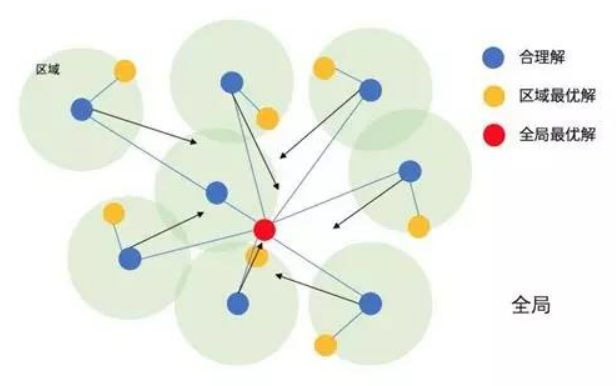
According to the game data of the hero League, this experiment builds a fully connected network classification model, optimizes the number of nodes and dropout probability of the neural network with particle swarm optimization algorithm, and finally compares the prediction accuracy of the default model and the optimized model on the game results of the hero LeagueParticle swarm optimization (PSO) is an evolutionary computing technology, which originates from the study of bird predation behavior. The basic idea of particle swarm optimization algorithm is to find the optimal solution through the cooperation and information sharing among individuals in the group. Its advantages are fast convergence and simple implementation, while its disadvantages are easy to fall into local optimization
Program / dataset Download
Click to enter the download address

code analysis
Import module
from tensorflow.keras.layers import Input,Dense,Dropout,Activation
import matplotlib.pyplot as plt
from tensorflow.keras.models import load_model
from tensorflow.keras.models import Model
from tensorflow.keras.optimizers import Adam
from sklearn.metrics import accuracy_score
import pandas as pd
import numpy as np
import json
from copy import deepcopy
The data is the 10 minute battle situation of each game of the hero League. The opponent of the hero League is divided into red and blue sides. blueWins refers to whether the blue side wins. Other columns are basically Bruce Lee, wild monster and economy. Forgive me for my unclear explanation... When I was in graduate school, I was promoted to silver. I had to be scolded every game because of the loading problem. By the way, I always installed girls and played auxiliary games in it, because there were fewer people scolding me. My friends were full. So it was not me that was wrong, but the world
data = pd.read_csv("Static/high_diamond_ranked_10min.csv").iloc[:,1:]
print("Data size:",data.shape)
print("Show the first 5 rows and columns of data")
data.iloc[:,:5].head()
Data size: (9879, 39)
Show the first 5 rows and columns of data
| blueWins | blueWardsPlaced | blueWardsDestroyed | blueFirstBlood | blueKills | |
|---|---|---|---|---|---|
| 0 | 0 | 28 | 2 | 1 | 9 |
| 1 | 0 | 12 | 1 | 0 | 5 |
| 2 | 0 | 15 | 0 | 0 | 7 |
| 3 | 0 | 43 | 1 | 0 | 4 |
| 4 | 0 | 75 | 4 | 0 | 6 |
Cut the data set into training, verification and testing. Here, only the verification set is used for PSO tuning, and the best checkpoint is not saved for neural network training
data = data.sample(frac=1.0)#Scramble data
trainData = data.iloc[:6000]#Training set
xTrain = trainData.values[:,1:]
yTrain = trainData.values[:,:1]
valData = data.iloc[6000:8000]#Validation set
xVal = valData.values[:,1:]
yVal = valData.values[:,:1]
testData = data.iloc[8000:]#Test set
xTest = testData.values[:,1:]
yTest = testData.values[:,:1]
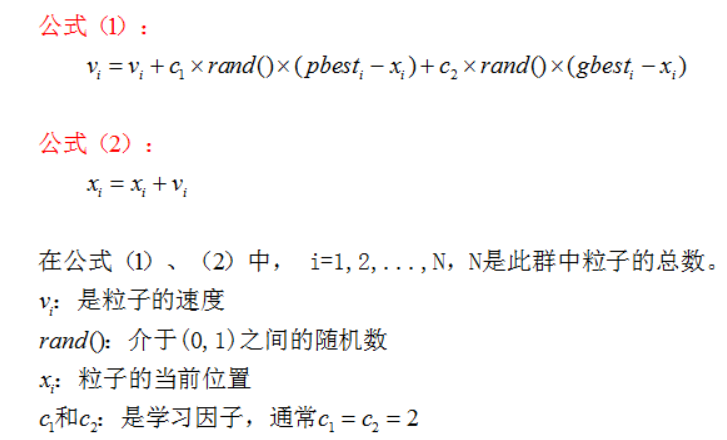
One particle is one scheme. In this experiment, one particle is an array (number of nodes and dropout probability). PSO is the process of calculating the fitness of each particle's corresponding scheme and finding the most suitable scheme. The following PSO class will iterate the particles according to the characteristics of the particles to be optimized, and support the characteristics of decimal or integer. If it is a self-determined discrete interval, it can be in the fitness function, The fitness of illegal particles is given a penalty value. After instantiating this class, it is necessary to specify the fitness function to iterate the particle scheme to the iterate function. The particle swarm optimization algorithm in this experiment is the simplest form, and the update formula is as follows:
class PSO():
    def __init__(self,featureNum,featureArea,featureLimit,featureType,particleNum=5,epochMax=10,c1=2,c2=2):
        '''
        Particle swarm optimization
        :param featureNum: Particle characteristic number
        :param featureArea: Characteristic upper and lower bound matrix
        :param featureLimit: The upper and lower boundary of the feature is also the opening and closing of the interval. 0 is excluded and 1 is included
        :param featureType: Feature type int float
        :param particleNum: Number of particles
        :param epochMax: Maximum number of iterations
        :param c1: Self cognitive learning factor
        :param c2: Group cognitive learning factor
        '''
        #As shown above
        self.featureNum = featureNum
        self.featureArea = np.array(featureArea).reshape(featureNum,2)
        self.featureLimit = np.array(featureLimit).reshape(featureNum,2)
        self.featureType = featureType
        self.particleNum = particleNum
        self.epochMax = epochMax
        self.c1 = c1
        self.c2 = c2
        self.epoch = 0#Number of iterations
        #Self optimal fitness record
        self.pBest = [-1e+10 for i in range(particleNum)]
        self.pBestArgs = [None for i in range(particleNum)]
        #Global optimal fitness record
        self.gBest = -1e+10
        self.gBestArgs = None
        #Initialize all particles
        self.particles = [self.initParticle() for i in range(particleNum)]
        #Initializes the learning speed of all particles
        self.vs = [np.random.uniform(0,1,size=featureNum) for i in range(particleNum)]
        #Iteration history
        self.gHistory = {"features%d"%i:[] for i in range(featureNum)}
        self.gHistory["Intra group average"] = []
        self.gHistory["global optimum "] = []

    def standardValue(self,value,lowArea,upArea,lowLimit,upLimit,valueType):
        '''
        Normalize an eigenvalue to fall within the interval
        :param value: characteristic value
        :param lowArea: lower limit
        :param upArea: upper limit
        :param lowLimit: Lower limit opening and closing interval
        :param upLimit: Upper limit opening and closing interval
        :param valueType: Feature type
        :return: Corrected value
        '''
        if value < lowArea:
            value = lowArea
        if value > upArea:
            value = upArea
        if valueType is int:
            value = np.round(value,0)

            #The lower limit is a closed interval
            if value <= lowArea and lowLimit==0:
                value = lowArea + 1
            #The upper limit is a closed interval
            if value >= upArea and upLimit==0:
                value = upArea - 1
        elif valueType is float:
            #The lower limit is a closed interval
            if value <= lowArea and lowLimit == 0:
                value = lowArea + 1e-10
            #Upper limit = closed
            if value >= upArea and upLimit==0:
                value = upArea - 1e-10
        return value

    def initParticle(self):
        '''Initialize 1 particle randomly'''
        values = []
        #Initialize so many features
        for i in range(self.featureNum):
            #Upper and lower limits of the feature
            lowArea = self.featureArea[i][0]
            upArea = self.featureArea[i][1]
            #The upper and lower bounds of this feature
            lowLimit = self.featureLimit[i][0]
            upLimit = self.featureLimit[i][1]
            #Random value
            value = np.random.uniform(0,1) * (upArea-lowArea) + lowArea
            value = self.standardValue(value,lowArea,upArea,lowLimit,upLimit,self.featureType[i])
            values.append(value)
        return values

    def iterate(self,calFitness):
        '''
        Start iteration
        :param calFitness:The input of fitness function is all features and global best fitness of a particle, and the output is fitness
        '''
        while self.epoch<self.epochMax:
            self.epoch += 1
            for i,particle in enumerate(self.particles):
                #The fitness of the particle
                fitness = calFitness(particle,self.gBest)
                #Update the particle's own cognitive best solution
                if self.pBest[i] < fitness:
                    self.pBest[i] = fitness
                    self.pBestArgs[i] = deepcopy(particle)
                #Update global best practices
                if self.gBest < fitness:
                    self.gBest = fitness
                    self.gBestArgs = deepcopy(particle)
            #Update particle
            for i, particle in enumerate(self.particles):
                #Update speed
                self.vs[i] = np.array(self.vs[i]) + self.c1*np.random.uniform(0,1,size=self.featureNum)*(np.array(self.pBestArgs[i])-np.array(self.particles[i])) + self.c2*np.random.uniform(0,1,size=self.featureNum)*(np.array(self.gBestArgs)-np.array(self.particles[i]))
                #Update eigenvalue
                self.particles[i] = np.array(particle) + self.vs[i]
                #Canonical eigenvalue
                values = []
                for j in range(self.featureNum):
                    #Upper and lower limits of the feature
                    lowArea = self.featureArea[j][0]
                    upArea = self.featureArea[j][1]
                    #The upper and lower bounds of this feature
                    lowLimit = self.featureLimit[j][0]
                    upLimit = self.featureLimit[j][1]
                    #Random value
                    value =self.particles[i][j]
                    value = self.standardValue(value,lowArea,upArea,lowLimit,upLimit,self.featureType[j])
                    values.append(value)
                self.particles[i] = values
            #Save historical data
            for i in range(self.featureNum):
                self.gHistory["features%d"%i].append(self.gBestArgs[i])
            self.gHistory["Intra group average"].append(np.mean(self.pBest))
            self.gHistory["global optimum "].append(self.gBest)
            print("PSO epoch:%d/%d Intra group average:%.4f global optimum :%.4f"%(self.epoch,self.epochMax,np.mean(self.pBest),self.gBest))
buildNet function constructs a simple fully connected classification network according to the number of network nodes and dropout probability. Its input feature number is 38 and the output feature number is 1 (of course, super parameters such as network layer number and learning rate can also be selected for optimization. In order to facilitate learning, only these two super parameters are selected for experiment) and trains the network
def buildNet(nodeNum,p):
    '''
    Build a fully connected network for training, return the model and training history, verify the accuracy of the set and test the accuracy of the set
    :param nodeNum: Number of network nodes
    :param p: dropout probability
    '''
    #38 game features of input layer
    inputLayer = Input(shape=(38,))

    #Middle layer
    middle = Dense(nodeNum)(inputLayer)
    middle = Dropout(p)(middle)

    #Output layer II Classification
    outputLayer = Dense(1,activation="sigmoid")(middle)

    #Model II Classification loss
    model = Model(inputs=inputLayer,outputs=outputLayer)
    optimizer = Adam(lr=1e-3)
    model.compile(optimizer=optimizer,loss="binary_crossentropy",metrics=['acc'])

    #train
    history = model.fit(xTrain,yTrain,verbose=0,batch_size=1000,epochs=100,validation_data=(xVal,yVal)).history

    #Validation set accuracy
    valAcc = accuracy_score(yVal,model.predict(xVal).round(0))
    #Test set accuracy
    testAcc = accuracy_score(yTest,model.predict(xTest).round(0))
    return model,history,valAcc,testAcc
In order to compare with the optimized model, we train a neural network with default parameters. Its super parameter value is the average value of each super parameter interval, and train and print the network structure and training index
nodeArea = [10,200]#Node number interval
pArea = [0,0.5]#dropout probability interval
#Training a neural network according to interval average
nodeNum = int(np.mean(nodeArea))
p = np.mean(pArea)
defaultNet,defaultHistory,defaultValAcc,defaultTestAcc = buildNet(nodeNum,p)
defaultNet.summary()
print("\n Number of nodes in the default network:%d dropout probability:%.2f Validation set accuracy:%.4f Test set accuracy:%.4f"%(nodeNum,p,defaultValAcc,defaultTestAcc))
Model: "model_346"
_________________________________________________________________
Layer (type)                 Output Shape              Param #
=================================================================
input_347 (InputLayer)       [(None, 38)]              0
_________________________________________________________________
dense_691 (Dense)            (None, 105)               4095
_________________________________________________________________
dropout_346 (Dropout)        (None, 105)               0
_________________________________________________________________
dense_692 (Dense)            (None, 1)                 106
=================================================================
Total params: 4,201
Trainable params: 4,201
Non-trainable params: 0
_________________________________________________________________

Number of nodes in the default network:105 dropout probability:0.25 Validation set accuracy:0.6535 Test set accuracy:0.6578
Instantiate the PSO model, input the interval information and start the iteration. The fitness function is to input 1 each particle and the global optimal fitness, and return the accuracy of the verification set of the corresponding scheme of the particle
featureNum = 2#2 features to be optimized
featureArea = [nodeArea,pArea]#2 characteristic value ranges
featureLimit = [[1,1],[0,1]]#The opening and closing of the value range 0 is the closed interval and 1 is the open interval
featureType = [int,float]#Type of 2 features
#Particle swarm optimization class
pso = PSO(featureNum,featureArea,featureLimit,featureType)
def calFitness(particle,gBest):
    '''Fitness function, input an array of particles and the global optimal fitness, and return the fitness corresponding to the particle'''
    nodeNum,p = particle#Take out the eigenvalues of particles
    net,history,valAcc,testAcc = buildNet(nodeNum,p)
    #The particle scheme exceeds the global optimum
    if valAcc>gBest:
        #Save model and corresponding information
        net.save("Static/best.h5")
        history = pd.DataFrame(history)
        history.to_excel("Static/best.xlsx",index=None)
        with open("Static/info.json","w") as f:
            f.write(json.dumps({"valAcc":valAcc,"testAcc":testAcc}))
    return valAcc
#Start swimming with particle swarm optimization
pso.iterate(calFitness)
#Load the best model and the corresponding training history
bestNet = load_model("Static/best.h5")
with open("Static/info.json","r") as f:
    info = json.loads(f.read())
bestValAcc = float(info["valAcc"])
bestTestAcc = float(info["testAcc"])
bestHistory = pd.read_excel("Static/best.xlsx")
print("Accuracy of verification set of optimal model:%.4f Test set accuracy:%.4f"%(bestValAcc,bestTestAcc))
PSO epoch:1/10 Intra group average:0.7210 global optimum :0.7280
PSO epoch:2/10 Intra group average:0.7210 global optimum :0.7280
PSO epoch:3/10 Intra group average:0.7251 global optimum :0.7280
PSO epoch:4/10 Intra group average:0.7275 global optimum :0.7350
PSO epoch:5/10 Intra group average:0.7275 global optimum :0.7350
PSO epoch:6/10 Intra group average:0.7299 global optimum :0.7350
PSO epoch:7/10 Intra group average:0.7313 global optimum :0.7350
PSO epoch:8/10 Intra group average:0.7313 global optimum :0.7350
PSO epoch:9/10 Intra group average:0.7313 global optimum :0.7350
PSO epoch:10/10 Intra group average:0.7313 global optimum :0.7350
 Accuracy of verification set of optimal model:0.7350 Test set accuracy:0.7350
View the transformation of PSO optimal solution with the number of iterations
history = pd.DataFrame(pso.gHistory)
history["epoch"] = range(1,history.shape[0]+1)
history
| Feature 0 | Feature 1 | Intra group average | global optimum | epoch | |
|---|---|---|---|---|---|
| 0 | 50.0 | 0.267706 | 0.7210 | 0.728 | 1 |
| 1 | 50.0 | 0.267706 | 0.7210 | 0.728 | 2 |
| 2 | 50.0 | 0.267706 | 0.7251 | 0.728 | 3 |
| 3 | 57.0 | 0.201336 | 0.7275 | 0.735 | 4 |
| 4 | 57.0 | 0.201336 | 0.7275 | 0.735 | 5 |
| 5 | 57.0 | 0.201336 | 0.7299 | 0.735 | 6 |
| 6 | 57.0 | 0.201336 | 0.7313 | 0.735 | 7 |
| 7 | 57.0 | 0.201336 | 0.7313 | 0.735 | 8 |
| 8 | 57.0 | 0.201336 | 0.7313 | 0.735 | 9 |
| 9 | 57.0 | 0.201336 | 0.7313 | 0.735 | 10 |
Comparing the accuracy of the default parameter model and PSO tuning model is a little effective, just for learning
fig, ax = plt.subplots()
x = np.arange(2)
a = [defaultValAcc,bestValAcc]
b = [defaultTestAcc,bestTestAcc]
total_width, n = 0.8, 2
width = total_width / n
x = x - (total_width - width) / 2
ax.bar(x, a,  width=width, label='val',color="#00BFFF")
for x1,y1 in zip(x,a):
    plt.text(x1,y1+0.01,'%.3f' %y1, ha='center',va='bottom')
ax.bar(x + width, b, width=width, label='test',color="#FFA500")
for x1,y1 in zip(x,b):
    plt.text(x1+width,y1+0.01,'%.3f' %y1, ha='center',va='bottom')
ax.legend()
ax.set_xticks([0,  1])
ax.set_ylim([0,1.2])
ax.set_ylabel("acc")
ax.set_xticklabels(["default net","PSO-net"])
fig.savefig("Static/contrast.png",dpi=250)
