Learning links: [Chinese] [Wu Enda's after class programming assignment] Course 1 - neural network and deep learning - assignment for the second week

○ operation objectives

What we need to do is build a simple neural network that can recognize cats

1, Use environment

Here, Anaconda is used for environment configuration and PyCharm is used for programming. Both can be downloaded by searching the official website.

-Package download

Here refer to the baidu online disk resources uploaded by the author in learning link 1
Data download , extraction code: 2u3w (if it fails, please go to the learning link above to see if the extraction code has been updated)

-Coding with Jupyter (only the opening method is mentioned here)

After installing Anaconda, open the "start" menu and find the location of Anaconda. You can find the built-in Jupiter notebook inside, which can be used. However, I don't think I can use it very well. I'd better use PyCharm seriously for coding. There will be no more mention here.

-Pre environment creation using Anaconda

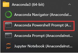
After installing anaconda, open Anaconda's console. I opened it in the start menu.

Step 1: create environment
In the console just opened, create a new environment using the following command:

conda create -n DeepLearning_wed python=3.8

Among them, DeepLearning_wed is your optional environment name.
You need to select Y/N during creation. Enter y and press enter.
Some common commands are introduced as follows:

conda info -e	#View currently owned environment
conda activate xxx	#Activate the environment named xxx (after activation, subsequent operations will be carried out in this environment)
conda list	#View what is installed in the current environment

Step 2: activate the environment
Activate with the following command:

conda activate DeepLearning_wed	#If your environment name is different from mine when you create it, please change the last string of characters to your environment name

2, Library installation

Before starting, the libraries to be introduced are (from learning link 1):

• numpy: it is a basic software package for scientific computing in Python.
• h5py: a common software package that interacts with data sets stored in H5 files.
• matplotlib: is a well-known library for drawing charts in Python.
• lr_utils: in the package of this article, a library of simple functions to load the data in the package.

Next, install one by one. Generally, first use conda search xxx to see if you can find the software to install. If you can find it, enter conda install xxx for installation.
Pre Description:
If you need to select y and n, please select y. Please don't hang the ladder to download, it will report an error!! If you think the download speed is too slow, you can search the Internet to hang the image source.

-numpy installation

conda search numpy	#Optional. If you need to view the version, you can enter this command to view it
conda install numpy	#Install numpy. If necessary, use "=" to specify the version number. If not specified, install the latest version

-Installation of h5py

conda search h5py	#Optional. If you need to view the version, you can enter this command to view it
conda install h5py	#Install h5py. If necessary, use "=" to specify the version number. If not specified, install the latest version

-Installation of matplotlib

conda search matplotlib	#Optional. If you need to view the version, you can enter this command to view it
conda install matplotlib	#Install matplotlib. If necessary, use "=" to specify the version number. If not specified, install the latest version

-lr_ Installation of utils

This is the tool in the given package and cannot be installed directly. Its import will be mentioned next.

3, Creation of programming environment

Step 1: create a project
Open PyCharm, select New project, and then operate as shown in the figure:

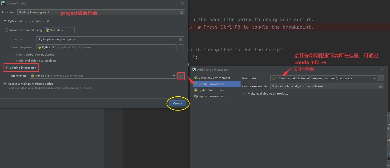
Select the Existing Interpreter, then click the three points on the right to select it, and then press OK. The Existing Interpreter will look like this:

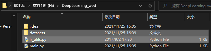
Step 2: put the folder downloaded from Baidu cloud into the directory where the project is located
As shown in the figure, the two selected are downloaded from Baidu cloud

Step 3: test whether all the completed environments are normal
You can copy the following code into main.py and run it

import numpy as np
import matplotlib.pyplot as plt
import h5py
from lr_utils import load_dataset

print('Hello,DeepLearning!')

If hello and deeplearning cannot be printed normally, please check which environment is not configured correctly.
To explain here, we will lr_utils can be imported through "from" in main.py only after it is placed in our project.

4, Learning process

-lr_ Explanation of contents in utils

lr_ The contents in utils are as follows:

import numpy as np
import h5py
    
    
def load_dataset():
    train_dataset = h5py.File('datasets/train_catvnoncat.h5', "r")
    train_set_x_orig = np.array(train_dataset["train_set_x"][:]) # your train set features
    train_set_y_orig = np.array(train_dataset["train_set_y"][:]) # your train set labels

    test_dataset = h5py.File('datasets/test_catvnoncat.h5', "r")
    test_set_x_orig = np.array(test_dataset["test_set_x"][:]) # your test set features
    test_set_y_orig = np.array(test_dataset["test_set_y"][:]) # your test set labels

    classes = np.array(test_dataset["list_classes"][:]) # the list of classes
    
    train_set_y_orig = train_set_y_orig.reshape((1, train_set_y_orig.shape[0]))
    test_set_y_orig = test_set_y_orig.reshape((1, test_set_y_orig.shape[0]))
    
    return train_set_x_orig, train_set_y_orig, test_set_x_orig, test_set_y_orig, classes

The following is referenced in learning link 1:
{
Explain the following above_ Meaning of the value returned by dataset():
train_set_x_orig: save the image data in the training set (this training set has 209 64x64 images).
train_set_y_orig: save the classification value corresponding to the image of the training set ([0 | 1], 0 means not a cat, and 1 means a cat).
test_set_x_orig: save the image data in the test set (this training set has 50 64x64 images).
test_set_y_orig: save the classification value corresponding to the image of the test set ([0 | 1], 0 means not a cat, and 1 means a cat).
classes: it saves two string data in bytes. The data is: [b'non-cat'b'cat '].
}

-View pictures in dataset

Through the above introduction lr_utils, we can know that the return value of the given function is train_ set_ x_ orig, train_ set_ y_ orig, test_ set_ x_ orig, test_ set_ y_ Orig and classes are variables.
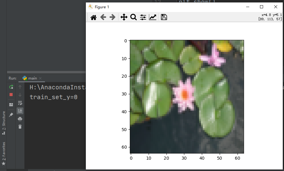
Let's try to print the picture on the screen.

import matplotlib.pyplot as plt
from lr_utils import load_dataset

#These variables are defined by load_ Returned in dataset()
train_set_x_orig , train_set_y , test_set_x_orig , test_set_y , classes = load_dataset()
index = 25  #The defined index value is 25
#We know train_set_x_orig stores pictures, which are array type data. Let's show the pictures
plt.imshow(train_set_x_orig[index])
#Let's print train_set_y_orig, look, is this a cat
print("train_set_y=" + str(train_set_y[0][25]))
#The next line is the code that really shows the picture on the screen
plt.show()

After running, the results are as follows:

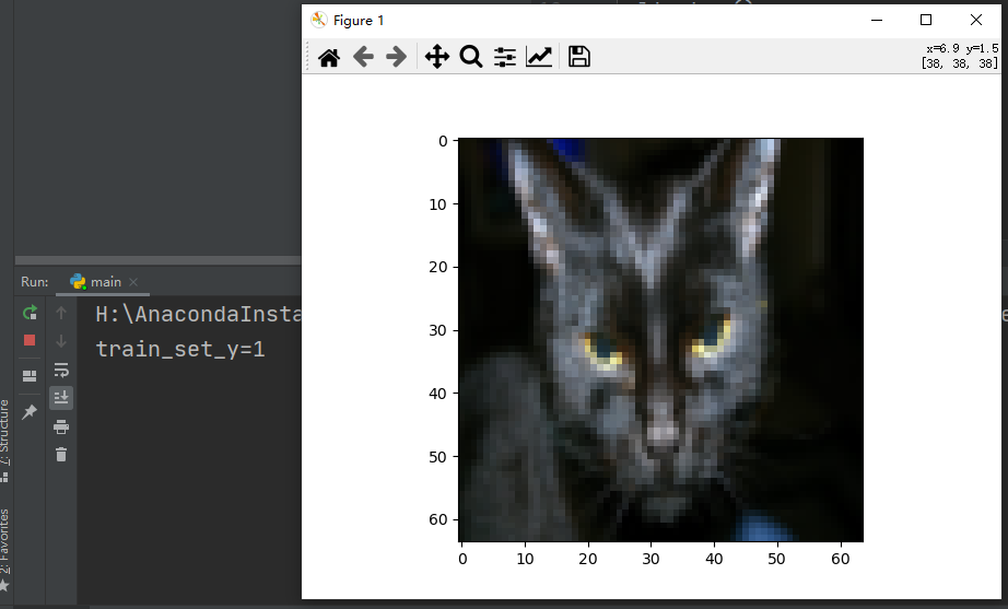
It can be seen from the picture that it is a cat, and the corresponding classification value is 1, indicating that it is a cat.
We change the index to 26, and the results are as follows:

That means it's not a cat.

-View and work with content in a dataset

The code here comes from the learning link, which will be personally understood on the basis of the learning link (which will be marked with {}).
{
Step 1: print train_set_y to view
Following the above content, we still use index=25

# Print out the current training tag value
# np.squeeze is used to compress dimensions, [uncompressed] train_ set_ The value of Y [:, index] is [1], and the value of [compressed] np.square (train_set_y[:,index]) is 1
print("[use np.squeeze: " + str(np.squeeze(train_set_y[:, index])) + "，Not used np.squeeze:  " + str(train_set_y[:, index]) + "]")
# Only the compressed value can be decoded
print("y=" + str(train_set_y[:, index]) + ", it's a " + classes[np.squeeze(train_set_y[:, index])].decode("utf-8") + " picture")

The printed result is: y = [1], it's a cat 'picture
Here I have a question about train_set_y[:, index] is not well understood.

Step 2: check the details of the image dataset
Next, let's take a look at the specific situation of the image dataset we loaded. I explain the following parameters:

• m_train: the number of pictures in the training set.
• m_test: the number of pictures in the test set.
• num_px: the width and height of the pictures in the training and test sets (both 64x64).

Remember, train_set_x_orig is an array with dimension (m_train, num_px, num_px, 3)

m_train = train_set_y.shape[1] #The number of pictures in the training set.
m_test = test_set_y.shape[1] #Number of pictures in the test set.
num_px = train_set_x_orig.shape[1] #The width and height of the pictures in the training and test sets (both 64x64).

#Now let's take a look at the details of what we loaded
print ("Number of training sets: m_train = " + str(m_train))
print ("Number of test sets : m_test = " + str(m_test))
print ("Width of each picture/high : num_px = " + str(num_px))
print ("Size of each picture : (" + str(num_px) + ", " + str(num_px) + ", 3)")
print ("Training set_Dimension of picture : " + str(train_set_x_orig.shape))
print ("Training set_Dimension of label : " + str(train_set_y.shape))
print ("Test set_Dimension of picture: " + str(test_set_x_orig.shape))
print ("Test set_Dimension of label: " + str(test_set_y.shape))

The results are:

Number of training sets: m_train = 209
 Number of test sets : m_test = 50
 Width of each picture/high : num_px = 64
 Size of each picture : (64, 64, 3)
Training set_Dimension of picture : (209, 64, 64, 3)
Training set_Dimension of label : (1, 209)
Test set_Dimension of picture: (50, 64, 64, 3)
Test set_Dimension of label: (1, 50)

Step 3: dimensionality reduction
For convenience, we need to reconstruct the numpy array with dimension (64, 64, 3) into an array with dimension (64 x 64 x 3, 1). The reason to multiply by 3 is that each picture is composed of 64x64 pixels, and each pixel is composed of (R, G, B) After that, our training and test data set is a numpy array, each column represents a flat image, and there should be m_train and m_test columns.

When you want to tile matrix X of shape (a, B, C, d) into matrix x_flat of shape (b * c * d, a), you can use the following code:

# X_flatten = X.reshape(X.shape [0], - 1).T X.T is the transpose of X
# Reduce and transpose the dimensions of the training set.
train_set_x_flatten = train_set_x_orig.reshape(train_set_x_orig.shape[0], -1).T
# Reduce and transpose the dimension of the test set.
test_set_x_flatten = test_set_x_orig.reshape(test_set_x_orig.shape[0], -1).T

This paragraph means to change the array into a matrix of 209 rows (because there are 209 pictures in the training set), but I am too lazy to calculate the number of columns, so I use - 1 to tell the program that you can help me calculate. When the program finally calculates 12288 columns, I finally use a T to represent transpose, which becomes 12288 rows and 209 columns. The same is true for the test set.
Print and see the results after dimensionality reduction:

print ("The last dimension of training set dimensionality reduction: " + str(train_set_x_flatten.shape))
print ("Training set_Dimension of label : " + str(train_set_y.shape))
print ("Dimension after dimension reduction of test set: " + str(test_set_x_flatten.shape))
print ("Test set_Dimension of label : " + str(test_set_y.shape))

The print result is:

The last dimension of training set dimensionality reduction: (12288, 209)
Training set_Dimension of label : (1, 209)
Dimension after dimension reduction of test set: (12288, 50)
Test set_Dimension of label : (1, 50)

To represent a color image, you must specify red, green, and blue channels (RGB) for each pixel Therefore, the pixel value is actually a vector of three numbers in the range from 0 to 255. A common preprocessing step in machine learning is to center and standardize the data set, which means that the average value of the whole numpy array in each example can be subtracted, and then each example can be divided by the standard deviation of the whole numpy array. However, for image data sets, it is simpler and more convenient , almost every row of the dataset can be divided by 255 (the maximum value of the pixel channel). Because there is no data larger than 255 in RGB, we can safely divide by 255 to make the standardized data between [0,1]. Now standardize our dataset:

train_set_x = train_set_x_flatten / 255
test_set_x = test_set_x_flatten / 255

}
Here, I would like to explain some vague points:
Why transpose: our target matrix is like this (see what the teacher said in the video): here n_x is the number of features of a sample, and m represents the total number of samples.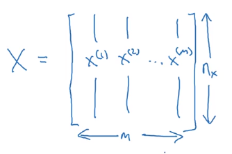
But obviously, before transposing, we get this: a row (n_x) is all the features of a sample, that is, the first column represents the first feature of all samples, the first column represents the second feature of all samples... And so on. At this time, the total number of samples (m) is the number of rows.

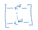
I think the blogger of the following figure source learning link 1 is well described:

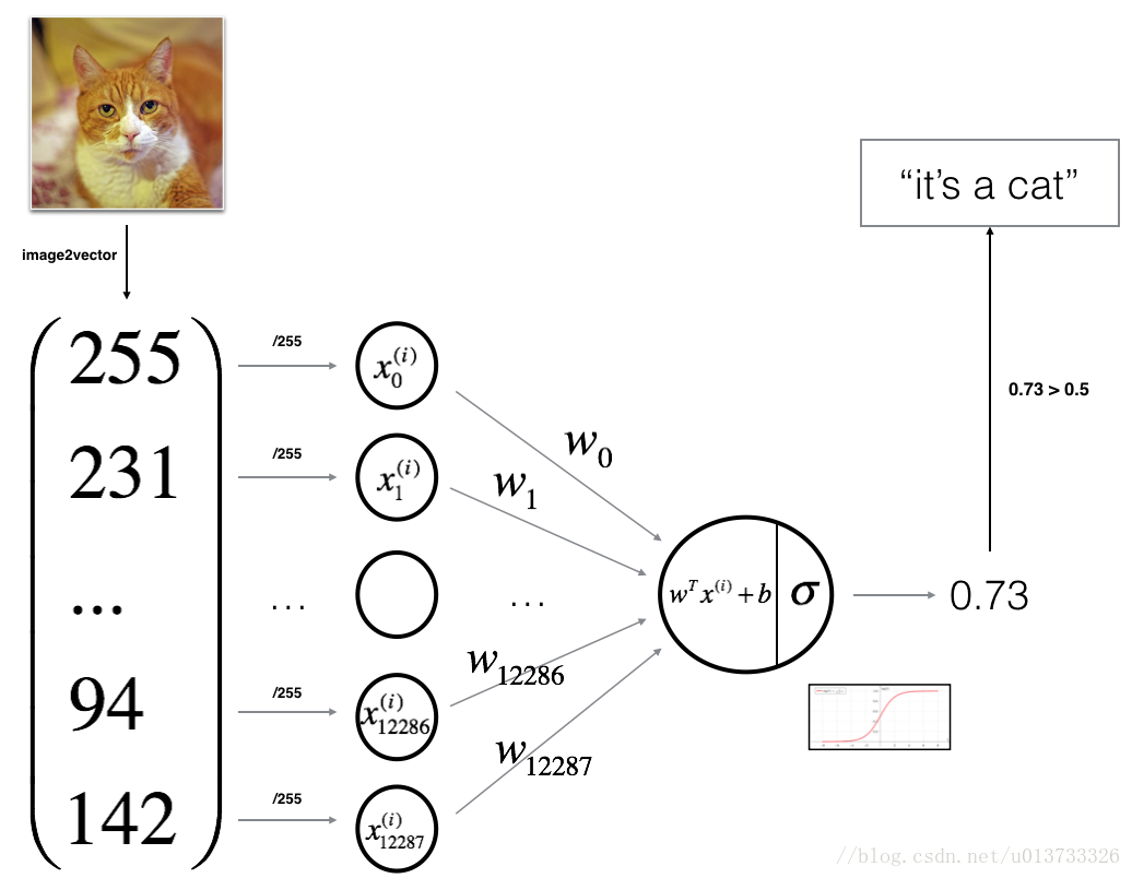
-Constructing neural network

Image source: learning link 1

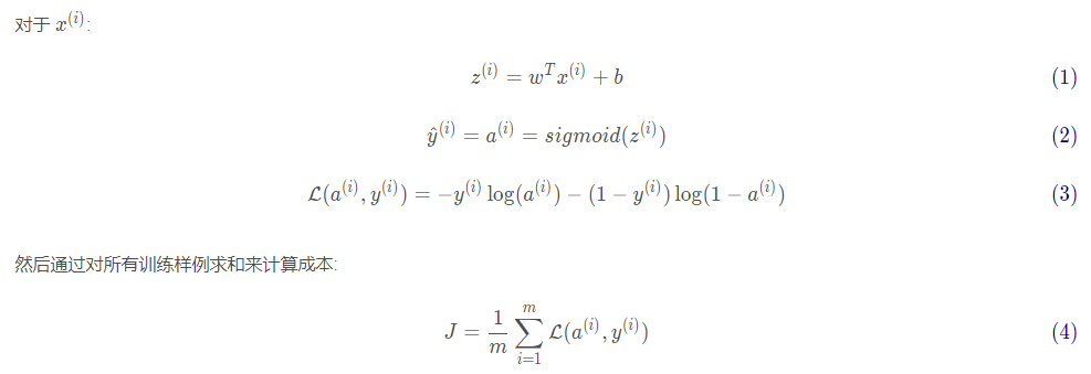
The main steps of establishing neural network are:

1. Define the structure of the model (for example, the number of input features)
2. Initialize the parameters of the model
3. Cycle:
   3.1 calculation of current loss (forward propagation)
   3.2 calculate current gradient (back propagation)
   3.3 update parameters (gradient descent)

Step 1: initialize parameters W and b

{

def initialize_with_zeros(dim):
    """
        This function is w Create a dimension for( dim，1)0 vector, and b Initialize to 0.

        Parameters:
            dim  - What we want w The size of the vector (or the number of parameters in this case)

        return:
            w  - Dimension is( dim，1)Initialization vector for.
            b  - Initialized scalar (corresponding to deviation)
    """
    w = np.zeros(shape=(dim, 1))
    b = 0
    # Use assert to ensure that the data I want is correct
    assert (w.shape == (dim, 1))  # The dimension of w is (dim,1)
    assert (isinstance(b, float) or isinstance(b, int))  # The type of b is float or int

    return (w, b)

}

Step 2: establish sigmoid function

{

def sigmoid(z):
    """
        Parameters:
            z  - Scalar or of any size numpy Array.

        return:
            s  -  sigmoid(z)
    """
    s = 1 / (1 + np.exp(-z))
    return s

The original author also did a test here. In fact, it's safer to do a test, but I'm in a hurry, so I won't do a test here.
}

Step 3: prepare for gradient descent (calculate dw and db)

{

def propagate(w, b, X, Y):
    m = X.shape[1]

    Z = np.dot(w.T + X) + b
    A = sigmoid(Z)
    cost = -(1/m) * np.sum(np.dot(Y, np.log(A)) + np.dot(1 - Y, np.log(1 - A)))

    dz = A - Y
    dw = (1 / m) * np.dot(X, dz.T)
    db = (1 / m) * np.sum(dz)

    assert (dw.shape == w.shape)
    assert (db.type == float)
    cost = np.squeeze(cost)
    assert (cost.shape == ())

    grads = {
        "dw": dw,
        "db": db
    }

    return (grads, cost)

}

Step 4: complete the gradient descent (that is, constantly update the values of w and b – call propagate())

{

def optimize(w, b, X, Y, num_irerations, learning_rate, print_cost=False):
    """
        This function is optimized by running the gradient descent algorithm w and b

        Parameters:
            w  - Weights, arrays of different sizes( num_px * num_px * 3，1)
            b  - Deviation, a scalar
            X  - Dimension is( num_px * num_px * 3，An array of training data.
            Y  - True label vector (0 if non cat, 1 if cat), matrix dimension(1,Number of training data)
            num_iterations  - Number of iterations of the optimization cycle
            learning_rate  - Learning rate of gradient descent update rule
            print_cost  - Print the loss value every 100 steps

        return:
            params  - Include weight w And deviation b Dictionary of
            grads  - A dictionary containing gradients of weights and deviations relative to the cost function
            cost - A list of all costs calculated during optimization will be used to draw the learning curve.

        Tips:
        We need to write down the following two steps and traverse them:
            1)Calculate the cost and gradient of the current parameter, using propagate(). 
            2)use w and b The gradient descent rule updates the parameters.
    """
    costs = []

    for i in num_irerations:

        grads, cost = propagate(w, b, X, Y)

        dw = grads["dw"]
        db = grads["db"]

        w = w - learning_rate * dw
        b = b - learning_rate * db

        # Record cost
        if i % 100 == 0:
            costs.append(cost)
        # Print cost data
        if (print_cost) and (i % 100 == 0):
            print("Number of iterations:%i ,   Error value:%f  " % (i, cost))

    params = {
        "w" : w,
        "b" : b
    }
    grads = {
        "dw" : dw,
        "db" : db
    }

    return (params, grads, costs)

}

Step 5: Forecast

{

The optimize function outputs the learned values of W and b. we can use w and b to predict the label of dataset X.
Now we are going to implement the prediction function predict(). There are two steps to calculate the prediction:

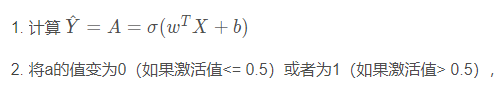
The predicted value is then stored in the vector Y_prediction.

def predict(w, b, X):
    """
        Using learning logistic regression parameters logistic (w，b)Whether the forecast tag is 0 or 1,

        Parameters:
            w  - Weights, arrays of different sizes( num_px * num_px * 3，1)
            b  - Deviation, a scalar
            X  - Dimension is( num_px * num_px * 3，Number of training data)

        return:
            Y_prediction  - contain X All predictions for all pictures in [0] | 1]One of numpy Array (vector)

    """
    m = X.shape[1]
    Y_prediction = np.zeros((1, m))
    w = w.reshape(X.shape[0], 1)

    # Calculate and predict the probability of cats appearing in the picture
    A = sigmoid(np.dot(w.T, X) + b)
    for i in (A.shape[1]):
        Y_prediction[0, i] = 1 if A[0, i] > 0.5 else 0
    assert(Y_prediction.shape == (1, m))

    return Y_prediction

}

Step 6: Integration

Complete all operations in one function:

def model(X_train, Y_train, X_test, Y_test, num_iterations = 2000, learning_rate = 0.5, print_cost = False):
    """
        Build the logistic regression model by calling the previously implemented functions

        Parameters:
            X_train  - numpy Array of,Dimension is( num_px * num_px * 3，m_train)Training set for
            Y_train  - numpy Array of,Dimension is (1, m_train)(Training label set for vector)
            X_test   - numpy Array of,Dimension is( num_px * num_px * 3，m_test)Test set for
            Y_test   - numpy Array of,Dimension is (1, m_test)Set of test tags for (vector)
            num_iterations  - A hyperparameter that represents the number of iterations used to optimize the parameter
            learning_rate  - express optimize()Update the superparameter of the learning rate used in the rule
            print_cost  - Set to true Print cost per 100 iterations

        return:
            d  - A dictionary that contains information about the model.
    """
    w, b = initialize_with_zeros(X_train.shape[0])

    parameters, grads, costs = optimize(w, b, X_train, Y_train, num_iterations, learning_rate, print_cost)

    w, b = parameters["w"], parameters["b"]

    Y_prediction_test = predict(w, b, X_test)
    Y_prediction_train = predict(w, b, X_train)

    # Print accuracy after training
    print("Training set accuracy:", format(100 - np.mean(np.abs(Y_prediction_train - Y_train)) * 100), "%")
    print("Test set accuracy:", format(100 - np.mean(np.abs(Y_prediction_test - Y_test)) * 100), "%")

    d = {
        "costs": costs,
        "Y_prediction_test": Y_prediction_test,
        "Y_prediciton_train": Y_prediction_train,
        "w": w,
        "b": b,
        "learning_rate": learning_rate,
        "num_iterations": num_iterations}
    return d

Step 7: call the code

d = model(train_set_x, train_set_y, test_set_x, test_set_y, num_iterations = 2500, learning_rate = 0.005, print_cost = True)

5, Supplement (from learning link 1)

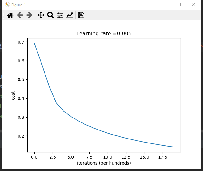
The chart of cost function can be printed out for viewing

#Drawing
costs = np.squeeze(d['costs'])
plt.plot(costs)
plt.ylabel('cost')
plt.xlabel('iterations (per hundreds)')
plt.title("Learning rate =" + str(d["learning_rate"]))
plt.show()

The results are as follows:

For further study, see the initial reference link.