All code for this experiment has been uploaded to your personal github repository: https://github.com/Scienthusiasts/Machine-Learning
Logistic Regression for Gesture Recognition
A long time ago, bloggers themselves had conceived a complete gesture recognition system with an interface, which could not only detect the gesture of the hand, but also determine the gesture of the hand corresponding to the information to be expressed. With this idea, you can do a lot of things, such as space drawing based on gestures, manipulating game scenes and so on (which can be combined with VR). In addition, you can control the mouse, control PPT page flipping, and so on. The application prospects of gesture-based recognition can be said to be very broad (or used for lesson setting). 🐛🐛🐛).
1. Ideas
The existing open source gesture recognition algorithms on the Internet are mainly based on two ideas:
One is to extract the contour or edge of the hand by image morphology, skin color detection, image filtering, and then extract the features of the hand based on the edge information.
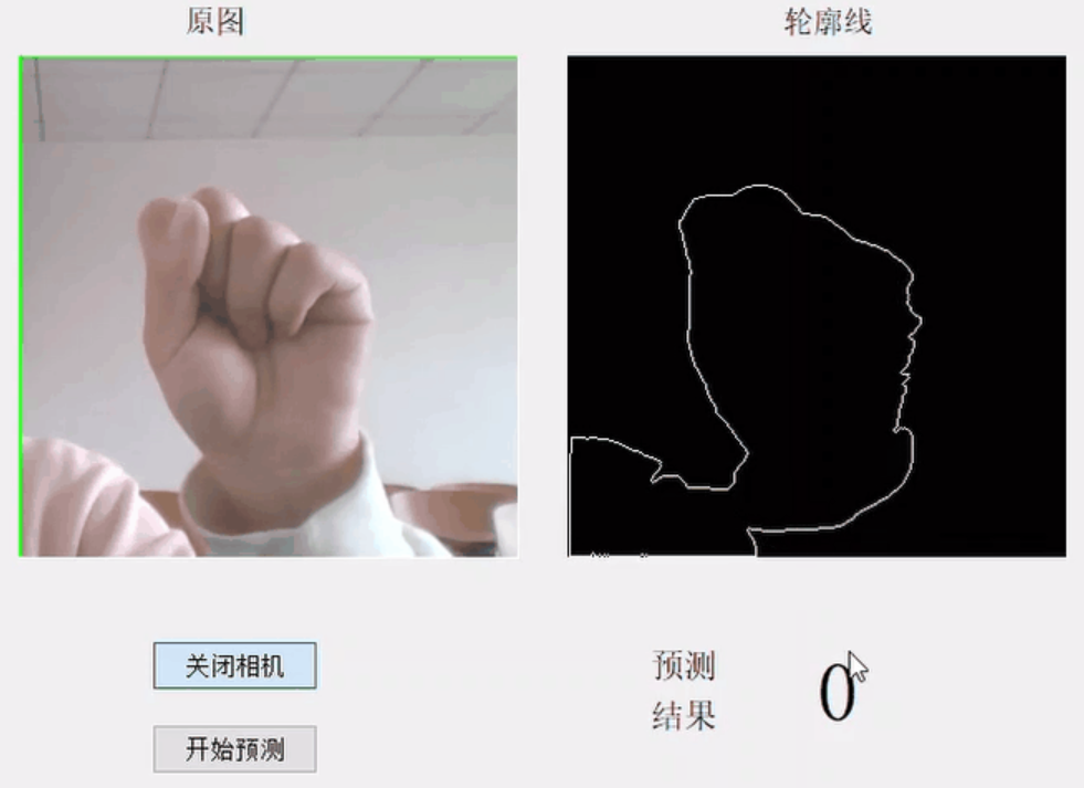
Image Source: OpenCV-based Gesture Recognition Complete Item (Python 3.7)
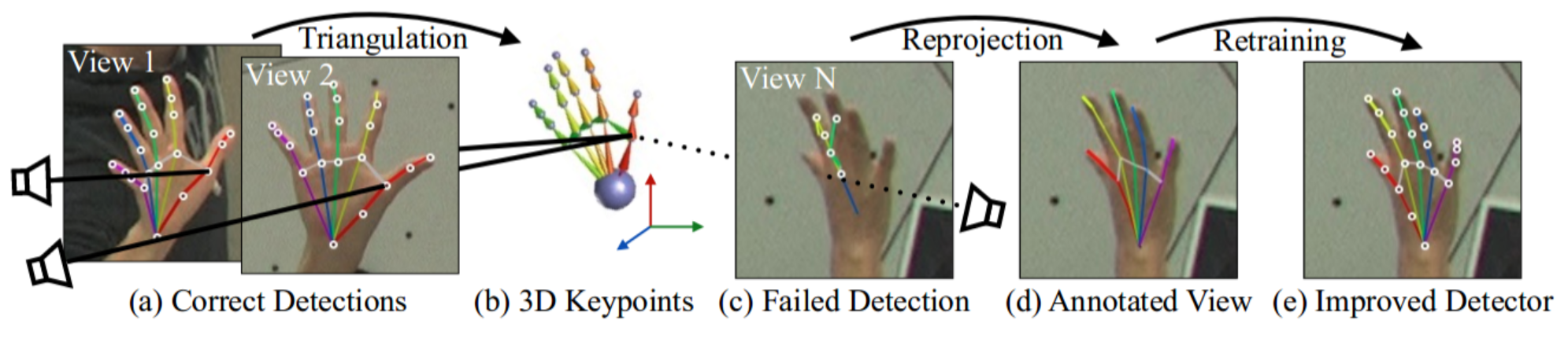
The other is to take the deep learning route, extract the hand area and key points through the deep network (which is also a regression + classification problem in nature), and then carry out routine operations (such as comparing angle between key points to judge posture, etc.). Or train a large number of gesture pictures directly based on the target detection algorithm, convolution neural network, which is similar to classic image recognition/target detection.
OpenPose-based detection of hand critical points:
In order to associate with the machine learning algorithms that the blogger is currently learning, in this blog, we will not consider how to achieve the regression of the hand key points, but only the classification. So the blogger will extract the hand key points based on the gesture detection algorithm in the Mediapipe Open Source Deep Learning Toolkit. Then we will classify the gestures based on these key points.
Meapipe hand key point detection consists of 21 hand key points:
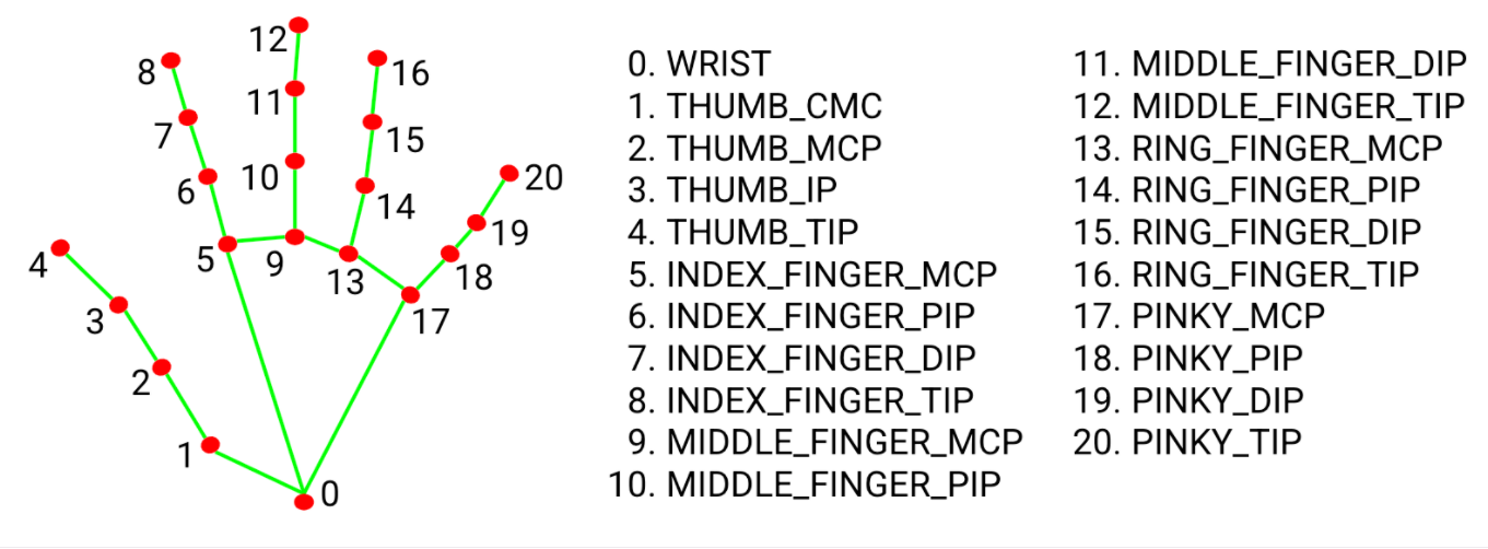
Mediapipe API Portal: https://google.github.io/mediapipe/solutions/hands
Some details
In fact, bloggers once thought about recording a large number of gesture images directly and then feeding them directly into the algorithm for training. But there are actually some problems: we know that images actually contain more detailed features than predictions made directly using key points, which in turn can cause too much noise. For a simple linear binary classification algorithm such as logistic regression, it may be difficult to train parameters with good generalization performance, so it may be a good strategy to select only hand key points as training data.
But how do we preprocess these key points to enable them to express posture information? The blogger's initial idea was to use the coordinates of the key points. However, the coordinates are absolute. If the positions of the hands in the image are different but the gestures are identical, their coordinates are also different, which adds an extra burden to the training of the algorithm. One idea is to use the distance between the key points, that is, the distance between two key points, as the dimension of the training data (this not only guarantees the translation invariance of the posture data, but also the rotation invariance: in three-dimensional coordinates, the distance between two key points of the same gesture at different angles is the same)
Okay, since the training data is selected, you can just do what you want, and the result will be good or not.
2. Implementation process
2.1 Data collection and pre-processing
2.1.1 Hand Key Point Extraction Based on the Meapipe Toolkit
The mediapipe website has provided us with a complete API and Python code implementation for hand key point detection. All we need to do is Ctrl C V, but some details need to be changed:
  ... ...
    if results.multi_hand_landmarks:
        for hand_landmarks in results.multi_hand_landmarks:
  ... ...
Below these two lines of related code are the extracted hand key points, and we can output hand_ Explore the landmarks variable:
... ...
landmark {
  x: 0.9662408828735352
  y: 0.5577888488769531
  z: -0.23717156052589417
}
... ...
Looking at it, you can see that hand_ There are 21 landmarks attributes under the landmarks variable, so we can conclude that each landmark corresponds to a key point of the hand, and that each landmark has three attributes, x, y and Z. This is clearly the spatial coordinate of each key point (the mediapipe integrated algorithm can predict the depth of the key point relative to the key point of the palm through a monocular camera). However, they are all in the (0,1) interval, so these coordinates should be normalized.
Code to extract coordinates:
... ...
keypoint = []
for i in range(21):
	x = hand_landmarks.landmark[i].x
	y = hand_landmarks.landmark[i].y
	z = hand_landmarks.landmark[i].z
    keypoint.append([x,y,z])
keypoint = np.array(keypoint)
... ...
Then remember the shape of the keypoint variable: [21,3]
It is obviously not enough to extract only one frame of gesture key points to train the algorithm, so for each gesture we extract 500 frames of key points and integrate them into a single dataset, store them in the position variable, and save them to a numpy binary file:
... ...
    if CNT<500:
        cv2.putText(image, str(CNT), (30,30), cv2.FONT_HERSHEY_SIMPLEX, .6, (0, 255, 0), 1)
        position.append(keypoint)
        CNT += 1
... ...
position = np.array(position)
print(position.shape)
np.save('./hand_frames.npy', position)
... ...
Then remember the shape of the position variable: [500,21,3]
Visualization of hand key points
The coordinates of the key points of the 500 frames of the hand are obtained, and the preprocessing can then be converted to the distance between the two key points. But before that, I thought it would be interesting to visualize these 500-frame keypoints first. 🤣
Visualization of hand key points:
# Draw gesture datasets over time
def draw(X, ax, step):
    lines = []
    # Draw lines between points
    lines.append(X[[0,1,2,3,4]])
    lines.append(X[[0,5,6,7,8]])
    lines.append(X[[0,17,18,19,20]])
    lines.append(X[[5,9,13,17]])
    lines.append(X[[9,10,11,12]])
    lines.append(X[[13,14,15,16]])
    for line in lines:
        ax.plot(line[:,0], line[:,1], line[:,2], linewidth=2)
        ax.set_xlim(0,1)
        ax.set_ylim(0,1)
        ax.set_zlim(-0.5,0.5)
    plt.pause(0.01)
    plt.cla()

# 3D Gesture Dataset Visualization
def show_frames(hand_frame):
    fig = plt.figure()
    # 3D Drawing
    ax = fig.add_subplot(111, projection='3d')
    for step, hand in enumerate(hand_frame):
        draw(hand, ax, step)
if __name__ == "__main__":
    # Recorded Gesture Dataset
    hand_frames = np.load('./hand_frame/hand_frame_one.npy')
    show_frames(hand_frames)
Visualizations (five fingers open on the left and two fists closed on the right):
[External chain picture transfer failed, source station may have anti-theft chain mechanism, it is recommended to save pictures and upload them directly (img-c2J0xqEU-1659868) (D:YHTLearningMachine LearningBlogLogistic Regression 4.gif)]
2.1.2 Converting absolute coordinates of key points to relative distances
When calculating distances, using numpy's broadcast mechanism, the distance matrix deal_between one key point and all other key points can be derived at once Hand_ Frame.py:
# Calculate the distance between a key point of a gesture and all points
def calc_dist(p1, p2):
    x = (p1[0]-p2[:,0]) * (p1[0]-p2[:,0])
    y = (p1[1]-p2[:,1]) * (p1[1]-p2[:,1])
    z = (p1[2]-p2[:,2]) * (p1[2]-p2[:,2])
    dist = x + y + z
    return dist

def distance(X):
    dataSets = []
    for hand in X:
        dist_matrix = []
        for i in range(21):
            dist_matrix.append(calc_dist(hand[i], hand))
        # plt.imshow(dist_matrix)
        # plt.pause(0.01)
        # plt.cla()
        dataSets.append(dist_matrix)
    return np.array(dataSets)
In addition, we can plot the distance between two critical points as a distance matrix, and we can visualize the distance matrix to see if there are any traceable features (which, to be honest, is not obvious). (The left image is the distance matrix with five fingers open and the right image is the distance matrix with two fists closed. These two datasets will be used as training sets for the Logistic Regression Bi-classification algorithm):
2.1.3 Building logistic Regression Algorithms
The principles of the logistic algorithm and the loss function I have described in relatively detail in the first two blogs, Machine Learning Algorithms. This experiment will not be covered anymore. Interested partners can check out the blogs I wrote in the first two articles.
Logistic regression algorithm code details logistic.py:
import sklearn.datasets as datasets # Dataset module
import numpy as np
import matplotlib.pyplot as plt
from sklearn.model_selection import train_test_split # Divide training set and validation set
import sklearn.metrics # sklearn evaluation module
from sklearn.preprocessing import StandardScaler # Standard Normalization
from sklearn.metrics import accuracy_score


# Setting Hyperparameters
LR= 1e-5         # learning rate
EPOCH = 20000   # Maximum number of iterations
BATCH_SIZE = 200  # Batch size


class logistic:
    def __init__(self, X=None, y=None, mode="pretrain"):
        self.X = X
        self.y = y
        # Record training loss, accuracy
        self.train_loss = []
        self.test_loss = []
        self.train_acc = []
        self.test_acc = []
        # Standard Normalization
        self.scaler = StandardScaler()
        # 1. Initialize W parameters
        if mode == "pretrain":
            self.W = np.load("../eval_param/Weight.npy")
        else:
            # Random Initialization W Parameter Initialization Parameter too large may cause too much loss and cause overflow
            self.W = np.random.rand(X.shape[1]+1, 1) * 0.1 # Uniform distribution size = [n,1] range [0,1]

    # Convert Probability to Category of Prediction
    def binary(self, y):
        y = y > 0.5
        return y.astype(int)


    # Binary sigmoid function
    def sigmoid(self, x):
        return 1/(1 + np.exp(-x))


    # Bi-classification cross-entropy loss
    def cross_entropy(self, y_true, y_pred):
        # Too close y_pred to 1 causes subsequent calculations np.log(1 - y_pred) = -inf
        crossEntropy = -np.sum(y_true * np.log(y_pred) + (1 - y_true) * np.log(1 - y_pred)) / (y_true.shape[0])
        return crossEntropy

    # Data preprocessing (training)
    def train_data_process(self):
        self.y = self.y.reshape(-1,1)
        # Divide training and validation sets using methods in sklearn
        X_train, X_test, y_train, y_test = train_test_split(self.X, self.y, test_size=0.3)
        # Standard Normalization
        self.std =  np.std(X_train, axis=0) + 1e-8
        self.mean = np.mean(X_train,axis=0)
        X_train = (X_train - self.mean) / self.std
        X_test = (X_test - self.mean) / self.std
        # Add offset
        X_train = np.concatenate((np.ones((X_train.shape[0], 1)), X_train), axis=1)
        X_test = np.concatenate((np.ones((X_test.shape[0], 1)), X_test), axis=1)
        # Number of batches per epoch
        NUM_BATCH = X_train.shape[0]//BATCH_SIZE+1
        print('Training Set Size:', X_train.shape[0], 'Validation Set Size:', X_test.shape[0])
        return X_train, X_test, y_train, y_test, NUM_BATCH


    def test_data_process(self, X):
        X = X.reshape(1,-1)
        # Standard Normalization
        self.std =  np.load('../eval_param/std.npy')
        self.mean = np.load('../eval_param/mean.npy')
        X = (X - self.mean) / self.std
        X = np.concatenate((np.ones((X.shape[0], 1)), X), axis=1)
        return X


    def train(self, LR, EPOCH, BATCH_SIZE):
        X_train, X_test, y_train, y_test, NUM_BATCH = self.train_data_process()
        for i in range(EPOCH):

            # This part of the code clutters the dataset, ensuring that each small iteration updates a different dataset
            # Produces a sequence of length m
            index = np.arange(X_train.shape[0])
            # The shuffle method randomly shuffles the sequence
            np.random.shuffle(index)
            # Disruption
            X_train = X_train[index]
            y_train = y_train[index]
            # Evaluate on the validation set:
            pred_y_test = self.sigmoid(np.dot(X_test, self.W))
            self.test_loss.append(self.cross_entropy(y_true=y_test, y_pred=pred_y_test))
            self.test_acc.append(accuracy_score(y_true=y_test, y_pred=self.binary(pred_y_test)))
            # On the training set:
            pred_y_train = self.sigmoid(np.dot(X_train, self.W))
            self.train_loss.append(self.cross_entropy(y_true=y_train, y_pred=pred_y_train))
            self.train_acc.append(accuracy_score(y_true=y_train, y_pred=self.binary(pred_y_train)))

            if i % BATCH_SIZE == 0:
                print("eopch: %d | train loss: %.6f | test loss: %.6f | train acc.:%.4f | test acc.:%.4f" %
                (i, self.train_loss[i], self.test_loss[i], self.train_acc[i], self.test_acc[i]))

            for batch in range(NUM_BATCH-1):
                # Slice operation to get corresponding batch training data (allow slices to exceed list range)
                X_batch = X_train[batch*BATCH_SIZE: (batch+1)*BATCH_SIZE]
                y_batch = y_train[batch*BATCH_SIZE: (batch+1)*BATCH_SIZE]

                # 2. To find the gradient, you need to derive W from the loss function corresponding to the multivariate linear regression above.
                previous_y = self.sigmoid(np.dot(X_batch, self.W))
                grad = np.dot(X_batch.T, previous_y - y_batch)

                # Add Regular Item
                # grad = grad + np.sign(W) # L1 Regular
                grad = grad + self.W            # L2 Regular

                # 3. Update parameters and use gradient descent formulas
                self.W = self.W - LR * grad


        # Print the final result
        for loop in range(32):
            print('===', end='')
        print("\ntotal iteration is : {}".format(i+1))
        y_hat_train = self.sigmoid(np.dot(X_train, self.W))
        loss_train = self.cross_entropy(y_true=y_train, y_pred=y_hat_train)
        print("train loss:{}".format(loss_train))
        y_hat_test = self.sigmoid(np.dot(X_test, self.W))
        loss_test = self.cross_entropy(y_true=y_test, y_pred=y_hat_test)
        print("test loss:{}".format(loss_test))
        print("train acc.:{}".format(self.train_acc[-1]))
        print("test acc.:{}".format(self.test_acc[-1]))


    def eval(self, X):
        X = self.test_data_process(X)
        y_hat = self.sigmoid(np.dot(X, self.W))
        return y_hat


    # Save weights
    def save(self):
        np.save("./eval_param/Weight.npy", self.W)
        np.save("./eval_param/std.npy", self.std)
        np.save("./eval_param/mean.npy", self.mean)

        np.save("./eval_param/train_loss.npy", self.train_loss)
        np.save("./eval_param/test_loss.npy", self.test_loss)
        np.save("./eval_param/train_acc.npy", self.train_acc)
        np.save("./eval_param.test_acc.npy", self.test_acc)
2.1.4 Training Details
import sklearn.datasets as datasets # Dataset module
import numpy as np
import matplotlib.pyplot as plt
from sklearn.model_selection import train_test_split # Divide training set and validation set
import sklearn.metrics # sklearn evaluation module
from sklearn.preprocessing import StandardScaler # Standard Normalization
from sklearn.metrics import accuracy_score


import sys;sys.path.append('../')
from logistic import logistic


if __name__ == "__main__":
    # Setting Hyperparameters
    LR= 1e-5         # learning rate
    EPOCH = 2000   # Maximum number of iterations
    BATCH_SIZE = 200  # Batch size

    # Import Dataset
    X1 = np.load("cloth_dist.npy")
    y1 = np.zeros(X1.shape[0])
    X2 = np.load("stone_dist.npy")
    y2 = np.ones(X1.shape[0])
    X  = np.concatenate((X1,X2), axis=0).reshape(-1,21*21)
    y  = np.concatenate((y1,y2), axis=0)

    model = logistic(X, y, mode="pretrain")

    model.train(LR, EPOCH, BATCH_SIZE)
    model.save()

    idx = 635
    print(model.eval(X[idx,:]), y[idx])
eopch: 0 | train loss: 12.153463 | test loss: 11.694130 | train acc.:0.0571 | test acc.:0.0667
eopch: 200 | train loss: 0.008306 | test loss: 0.007973 | train acc.:0.9986 | test acc.:1.0000
... ...
eopch: 2000 | train loss: 0.000877 | test loss: 0.000713 | train acc.:1.0000 | test acc.:1.0000
================================================================================================
total iteration is : 2000
train loss:0.0008687095801340618
test loss:0.0007078273117643203
train acc.:1.0
test acc.:1.0
You can see that the test results of the final model on the validation set are unexpectedly good. Next, let's see how the generalization performance of the model is.
2.1.5 algorithm test (embedded in mediapipe hand key point extraction code)
Simply add these lines of code under the Extract Code at the critical point of your hand (remember to import your custom package):
... ...
from deal_hand_frame import distance
import sys;sys.path.append('../')
from logistic import logistic
... ...
      X = distance(keypoint.reshape(1,21,3)).reshape(-1)
        # print(int(model.eval(X)>0.5))
        cls = {0:'cloth', 1:"fist"}
        cv2.putText(image, cls[int(model.eval(X)>0.5)], (200,50), cv2.FONT_HERSHEY_SIMPLEX, 2, (0, 0, 255), 3)
... ...
The final algorithm is based on real-time camera recognition or very Robust:
3. Algorithm Improvement
In 2.1.2, it is not difficult to find that there is redundancy in calculating the distance between two key points, such as the distance between key point 1 and 6 is exactly the same as that between key point 6 and key point 1. Therefore, the distance matrix obtained by the current algorithm is a symmetric matrix and will be improved in the future. We can only select the upper triangle of the distance matrix.
Also, the distance between the key point itself and itself must be 0, so the dimensions on the principal diagonal of the distance matrix can be discarded. In addition, the distance between two key points of adjacent joints of the hand must be the same in reality (unless you dislocate them), so disturbances in the distance between these key points can only exist as noise. These dimensions can also be removed in subsequent algorithm improvements.