catalogue

1, Basic concept of regression

2, Classification based on Logistic regression and Sigmoid function

3, Determination of optimal regression coefficient based on optimization method

1. Maximum likelihood estimation Recap

2. Gradient rise method

3. Prepare data: a simple data set

4. Training algorithm: use gradient rise to find the best parameters

5. Analyze data: draw decision boundaries

6. Training algorithm: random gradient rising algorithm

7. Improved random gradient rise algorithm

4, Example: predicting mortality of diseased horses from hernia symptoms

1. Preparing data: Processing missing values in data

2. Test algorithm: use gradient rise algorithm for classification

3. Test algorithm: the improved random gradient rise algorithm is used for classification

4. Example: practice summary

1, Basic concept of regression

         For some existing data points, we use a straight line to fit these points, which is called the best fitting straight line, and this fitting process is called regression. The main idea of using Logistic regression for classification is to establish a regression formula for the classification boundary line according to the existing data. The word "regression" here comes from the best fitting, which means to find the best fitting parameter set. The method of training classifier is to find the best fitting parameters, and the optimization algorithm is used.

General process of Logistic regression

(1) Data collection: collect data by any method. (2) Prepare data: since distance calculation is required, the data type is required to be numerical. In addition, the structured data format is the best. (3) Analyze data: analyze the data by any method. (4) Training algorithm: most of the time will be used for training. The purpose of training is to find the best classification regression coefficient. (5) Test algorithm: once the training steps are completed, the classification will be fast. (6) Using algorithm: first, we need to input some data and convert it into corresponding structured values; Then, based on the trained regression coefficients, these values can be simply regressed to determine which category they belong to; After that, we can do some other analysis work on the output categories.

2, Classification based on Logistic regression and Sigmoid function

Logistic regression

Advantages: low computational cost, easy to understand and implement. Disadvantages: it is easy to under fit, and the classification accuracy may not be high. Applicable data types: numerical data and nominal data.

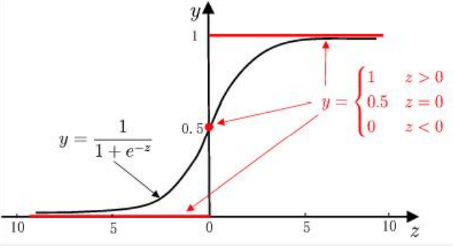
         Logistic regression is used to solve the classification problem. The function we want should be able to accept all inputs and predict the category. For example, in the case of two classes, the above function outputs 0 or 1. For example, the Heaviside step function, also known as the unit step function.

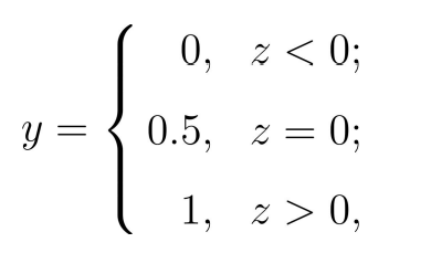
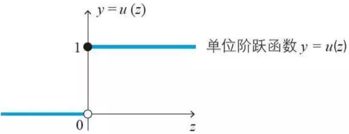
         The problem of hevised step function is that it jumps from 0 to 1 (discontinuous and non differentiable) at the jump point, which is sometimes difficult to deal with. But mathematically, the Sigmoid function can solve this problem. The specific calculation formula of Sigmoid function is as follows:

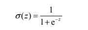
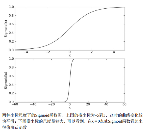
         The following figure shows two curves of Sigmoid function under different coordinate scales. When x is 0, the Sigmoid function value is 0.5. With the increase of X, the corresponding Sigmoid value will approach 1; With the decrease of X, the Sigmoid value will approach 0. If the abscissa scale is large enough, the Sigmoid function looks like a step function.

         Therefore, in order to realize Logistic regression classification, we can multiply each feature by a regression coefficient, then add all the result values, and substitute the sum into the Sigmoid function to obtain a value ranging from 0 to 1. Any data greater than 0.5 is classified as class 1, and less than 0.5 is classified as class 0. Therefore, Logistic regression can also be regarded as a probability estimation.

Predicted value and output flag: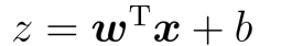   
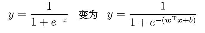
The input value of Sigmoid function is z, vector x is the input data of the classifier, vector w is the best coefficient found, and b is a constant.

Using the Sigmoid function:

  log odds: the logarithm of the relative probability of the sample as a positive example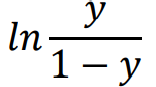  

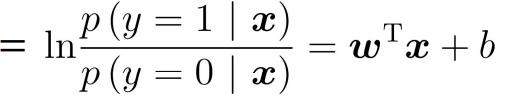
  Therefore:

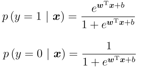
The above two formulas represent the probabilities of y=1 and y=0 respectively. adopt, we obtain the z value, and then map the z value to 0 ~ 1 through the Sigmoid function. After obtaining the value, we can classify it. For example, by definition, the classification greater than 0.5 is 1, otherwise, the classification is 0. Therefore, the problem we need to solve is to obtain the best regression coefficient, that is, to solve the values of w and b.

3, Determination of optimal regression coefficient based on optimization method

1. Maximum likelihood estimation Recap

① Method steps of maximum likelihood estimation

• Determine unknown parameters to be solved, such as mean, variance or parameters of specific distribution function;
• Calculate each sampleThe probability density of is；
• The likelihood function is constructed according to the cumulative multiplication of the probability density of the sample:
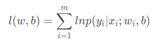
• The unknown parameters are solved by maximizing the likelihood function (derivative is 0) θ， In order to reduce the difficulty of calculation, logarithmic addition can be used to replace probability multiplication, and the unknown parameters can be solved by derivative of 0 / maximum.

② Maximizing the probability that a sample belongs to its true marker is equivalent to maximizing the log likelihood function:

③ Transformed into maximized logistic likelihood function solution:
，

④ According to the sigmoid function, the likelihood function can be rewritten as:

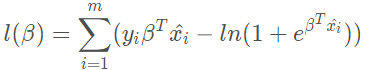
  Therefore, the equivalent form is to minimize the equation.

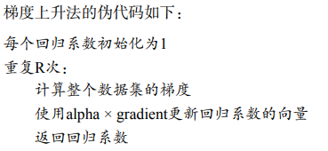
2. Gradient rise method

          The idea of gradient rising method is that the best way to find the maximum value of a function is to explore along the gradient direction of the function. If the gradient is written as ≓, the gradient of function f(x,y) is expressed by the following formula:

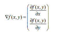
This gradient means moving in the direction of x , move in the direction of y . The function f(x,y) must be defined and differentiable at the point to be calculated. As shown below:

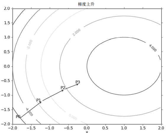
        As shown in the figure, the gradient rise algorithm will re estimate the moving direction after reaching each point. Starting from P0, after calculating the gradient of this point, the function moves to the next point P1 according to the gradient. At P1, the gradient is recalculated again and moved to P2 along the new gradient direction. This cycle iterates until the stop condition is met. In the process of iteration, the gradient operator always ensures that we can select the best moving direction.

         The gradient rise algorithm moves one step along the gradient direction. It can be seen that the gradient operator always points to the direction where the value of the function increases the fastest. What is said here is the moving direction, not the size of the moving amount. This value is called step size and is recorded as α. In terms of vector, the iterative formula of gradient rise algorithm is as follows:

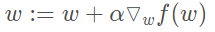
         The formula will be executed iteratively until a stop condition is reached, such as the number of iterations reaches a specified value or the algorithm reaches an allowable error range.

Gradient descent algorithm

The gradient descent algorithm is the same as the gradient rise algorithm here, except that the addition in the formula needs to become subtraction. Therefore, the corresponding formula can be written as:

  The gradient rise algorithm is used to find the maximum value of the function, and the gradient fall algorithm is used to find the minimum value of the function.

3. Prepare data: a simple data set

Data of testSet.txt

X1	X2	Classification label
0.355715	10.325976	0
-1.39563	4.662541	1
-0.75216	6.53862	0
-1.32237	7.152853	0
......	······	······
1.985298	3.230619	1
-1.69345	-0.55754	1
-0.57653	11.77892	0
-0.34681	-1.67873	1
-2.12448	2.672471	1

         There are 100 sample points, and each point contains two numerical features: X1 and X2. On this data set, the best regression coefficient is found by using the gradient rise method, that is, the best parameters of the Logistic regression model are fitted.

# Load dataset
def loadDataSet():
    dataMat = []                                                      # Data list
    labelMat = []                                                     # Tag list
    fr = open('testSet.txt')                                          # Open file
    for line in fr.readlines():                                       # Traverse each row and read the data
        lineArr = line.strip().split()                                # Remove carriage return
        dataMat.append([1.0, float(lineArr[0]), float(lineArr[1])])   # Add the data of this row to the data list
        labelMat.append(int(lineArr[2]))                              # Add tag to list
    return dataMat, labelMat

# Draw dataset
def showData():
    dataMat, labelMat = loadDataSet()                      # Loading datasets, labels
    dataArr = array(dataMat)                               # Array converted to umPy
    n = shape(dataArr)[0]                                  # Total number of acquired data
    xcord1 = []; ycord1 = []                               # Store positive samples
    xcord2 = []; ycord2 = []                               # Store negative samples
    for i in range(n):                                     # Classify the data according to the label of the data set
        if int(labelMat[i]) == 1:                          # The label of the data is 1, indicating a positive sample
            xcord1.append(dataArr[i, 1]); ycord1.append(dataArr[i, 2])
        else:                                              # Otherwise, if the label of the data is not 1, it represents a negative sample
            xcord2.append(dataArr[i, 1]); ycord2.append(dataArr[i, 2])
    fig = plt.figure()
    ax = fig.add_subplot(111)
    ax.scatter(xcord1, ycord1, s=15, c='blue')             # Draw positive samples
    ax.scatter(xcord2, ycord2, s=15, c='red', marker='s')  # Draw negative samples
    plt.title('DateSet')                                   # title
    plt.xlabel('X1'); plt.ylabel('X2')                     # x. Label for y-axis
    plt.show()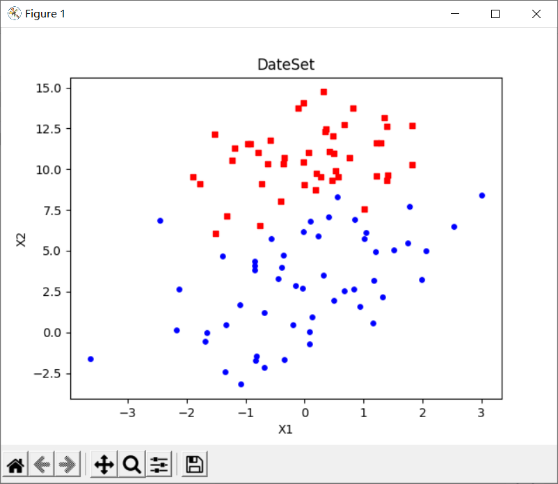

4. Training algorithm: use gradient rise to find the best parameters

     

# sigmoid function
def sigmoid(inX):
    return 1.0 / (1 + exp(-inX))

# Gradient rise algorithm
def gradAscent(dataMatIn, classLabels):                            # dataMatIn dataset, classLabels data labels
    dataMatrix = mat(dataMatIn)                                    # Convert to NumPy matrix
    labelMat = mat(classLabels).transpose()                        # Convert to NumPy matrix and transpose the matrix
    m, n = shape(dataMatrix)                                       # Gets the size of the dataset matrix. m is the number of rows and n is the number of columns
    alpha = 0.001                                                  # Step size of target movement
    maxCycles = 500                                                # Number of iterations
    weights = ones((n, 1))                                         # The weight is initialized to 1
    for k in range(maxCycles):                                     # Repeated matrix operation
        h = sigmoid(dataMatrix * weights)                          # Matrix multiplication to calculate sigmoid function
        error = (labelMat - h)                                     # calculation error
        weights = weights + alpha * dataMatrix.transpose() * error # Matrix multiplication to update weight
    return weights

# Obtain regression coefficient
dataMat, labelMat = loadDataSet()
weigths = gradAscent(dataMat, labelMat)
print("w0: %f, w1: %f, W2: %f" % (weigths[0], weigths[1], weigths[2]))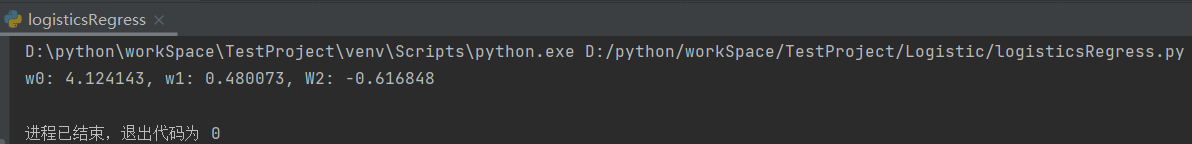

  

5. Analyze data: draw decision boundaries

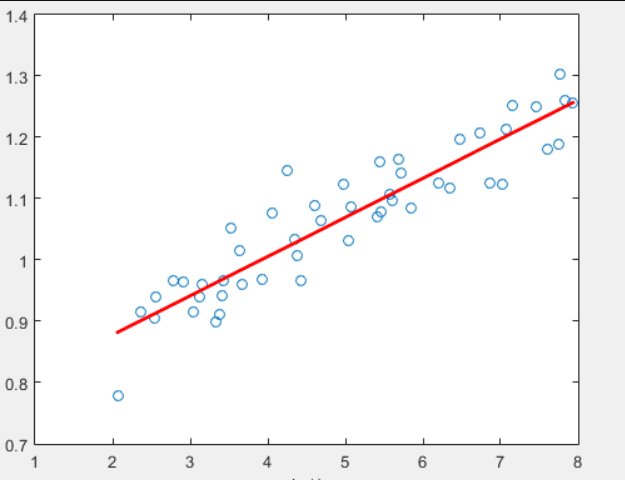
          A set of regression coefficients has been solved above, which determines the separation line between different categories of data. Now we can try to draw this separation line,

# Draw the best fitting line of data set and Logistic regression
def plotBestFit(weights):
    dataMat, labelMat = loadDataSet()                      # Loading datasets, labels
    dataArr = array(dataMat)                               # Array converted to umPy
    n = shape(dataArr)[0]                                  # Total number of acquired data
    xcord1 = []; ycord1 = []                               # Store positive samples
    xcord2 = []; ycord2 = []                               # Store negative samples
    for i in range(n):                                     # Classify the data according to the label of the data set
        if int(labelMat[i]) == 1:                          # The label of the data is 1, indicating a positive sample
            xcord1.append(dataArr[i, 1]); ycord1.append(dataArr[i, 2])
        else:                                              # Otherwise, if the label of the data is not 1, it represents a negative sample
            xcord2.append(dataArr[i, 1]); ycord2.append(dataArr[i, 2])
    fig = plt.figure()
    ax = fig.add_subplot(111)
    ax.scatter(xcord1, ycord1, s=30, c='red', marker='s')  # Draw positive samples
    ax.scatter(xcord2, ycord2, s=30, c='green')            # Draw negative samples
    x = arange(-3.0, 3.0, 0.1)                             # x interval
    y = (-weights[0] - weights[1] * x) / weights[2]        # Best fit line
    ax.plot(x, y)
    plt.title('BestFit')                                   # title
    plt.xlabel('X1'); plt.ylabel('X2')                     # x. Label for y-axis
    plt.show()

# Operation drawing
dataMat, labelMat = loadDataSet()
weigths = gradAscent(dataMat, labelMat)
plotBestFit(weigths.getA())
print("w0: %f, w1: %f, W2: %f" % (weigths[0], weigths[1], weigths[2]))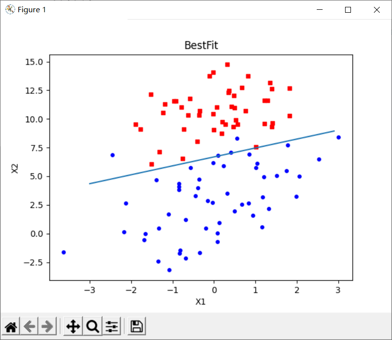

          From the result graph, we can see that the classification result is very good. From the graph, there are not many wrong points. However, although the example is simple and the data set is small, this method requires 300 multiplications and a lot of calculation.

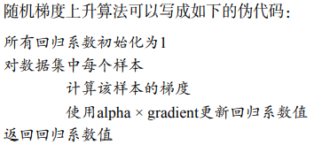
6. Training algorithm: random gradient rising algorithm

         The gradient rise algorithm needs to traverse the whole data set every time the regression coefficient is updated. This method is feasible when dealing with about 100 data sets, but if there are billions of samples and thousands of features, the computational complexity of this method is too high. An improved method is to update the regression coefficient with only one sample point at a time. This method is called random gradient rise algorithm. Because the classifier can be updated incrementally when new samples arrive, the random gradient rise algorithm is an online learning algorithm. Corresponding to "online learning", processing all data at once is called "batch processing".

# Random gradient rise algorithm
def stocGradAscent0(dataMatrix, classLabels):              # dataMatIn dataset, classLabels data labels
    m, n = shape(dataMatrix)                               # Gets the size of the dataset matrix. m is the number of rows and n is the number of columns
    alpha = 0.01                                           # Step size of target movement
    weights = ones(n)                                      # So initialize to 1
    for i in range(m):                                     # Repeated matrix operation
        h = sigmoid(sum(dataMatrix[i] * weights))          # Matrix multiplication to calculate sigmoid function
        error = classLabels[i] - h                         # calculation error
        weights = weights + alpha * error * dataMatrix[i]  # Matrix multiplication to update weight
    return weights

         It can be seen that the random gradient rise algorithm is very similar to the gradient rise algorithm in code, but there are some differences: first, the variable h and error error of the latter are vectors, while the former is all numerical values; Second, the former has no matrix conversion process, and the data types of all variables are NumPy arrays.

# Run test code
dataMat, labelMat = loadDataSet()
weigths = stocGradAscent0(array(dataMat), labelMat)
plotBestFit(weigths)
print("w0: %f, w1: %f, W2: %f" % (weigths[0], weigths[1], weigths[2]))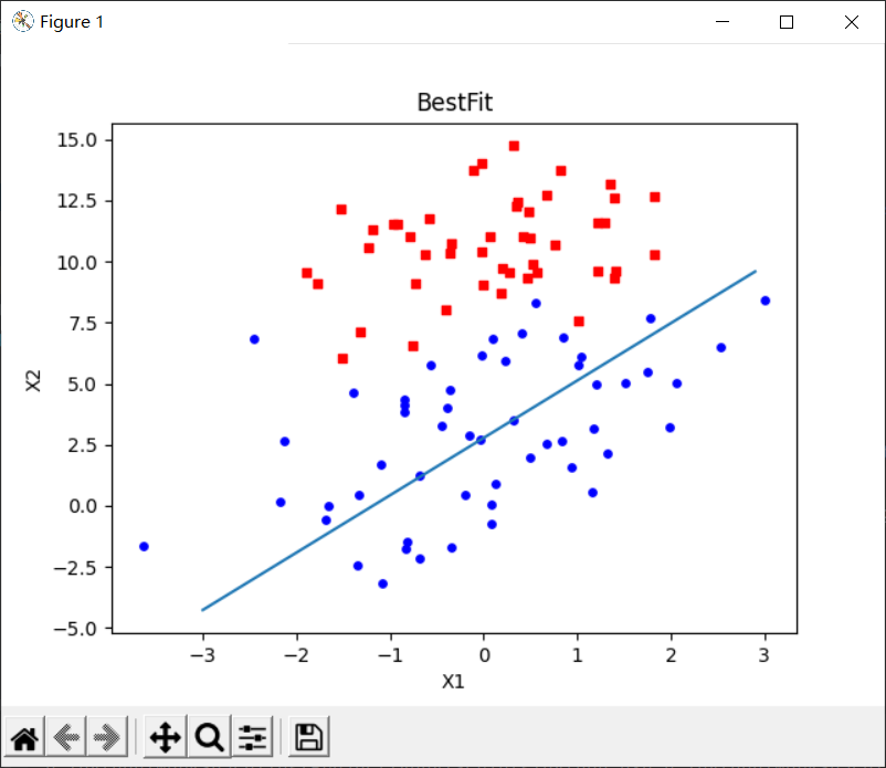

         According to the execution results of the random gradient rise algorithm on the above data sets, the best fitting line is not the best classification line, and it can be seen that there is a great deviation in the fitting curve.

        As shown in the figure above, the change of regression coefficient of random gradient rise algorithm during 200 iterations is shown. X2 in the figure above has reached the stable value after only 50 iterations, but X1 and X0 need more iterations. After the big fluctuations stop, there are some small periodic fluctuations. The reason for this phenomenon is that there are some sample points that can not be classified correctly, which will cause drastic changes in the coefficients during each iteration.  

7. Improved random gradient rise algorithm

# Improved random gradient rise algorithm
def stocGradAscent1(dataMatrix, classLabels, numIter=150):  # dataMatIn dataset, classLabels, numIter iterations
    m, n = shape(dataMatrix)                                # Gets the size of the dataset matrix. m is the number of rows and n is the number of columns
    weights = ones(n)                                       # So initialize to 1
    for j in range(numIter):
        dataIndex = list(range(m))                          # Create data index list
        for i in range(m):
            alpha = 4 / (1.0 + j + i) + 0.0001              # The step length of apha target movement is adjusted each iteration
            randIndex = int(random.uniform(0, len(dataIndex)))  # Randomly selected update samples
            h = sigmoid(sum(dataMatrix[randIndex] * weights))   # Matrix multiplication to calculate sigmoid function
            error = classLabels[randIndex] - h                  # calculation error
            weights = weights + alpha * error * dataMatrix[randIndex]  # Matrix multiplication to update weight
            del (dataIndex[randIndex])                                 # Delete used samples
    return weights

# test
dataMat, labelMat = loadDataSet()
weigths = stocGradAscent1(array(dataMat), labelMat)
plotBestFit(weigths)
print("w0: %f, w1: %f, W2: %f" % (weigths[0], weigths[1], weigths[2]))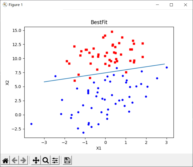

         The first aspect of improvement is alpha = 4 / (1.0 + j + i) + 0.0001. Alpha will be adjusted at each iteration. In addition, although alpha will decrease with the number of iterations, it will never decrease to 0. The reason for this is to ensure that the new data still has an impact after multiple iterations. If the problem to be dealt with is dynamic, the above constant term can be appropriately increased to ensure that the new value obtains a larger regression coefficient. Another point worth noting is that in the function of reducing alpha, alpha is reduced by 1/(j+i) each time, where j is the number of iterations and i is the subscript of the sample point.

        The second improvement is at randindex = int (random. Uniform (0, len (dataindex)). Here, the regression coefficient is updated by randomly selecting samples. Each time, the sample points are unused in the iteration. This method will reduce the periodic fluctuation and reduce the amount of calculation. Moreover, it can be seen from the above operation results that the regression effect is very good.  

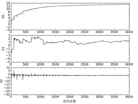
        As shown in the figure above, the coefficient convergence diagram generated by the random gradient rise algorithm stocGradAscent1() using sample random selection and alpha dynamic reduction mechanism. This method converges faster than the fixed alpha method.

4, Example: predicting mortality of diseased horses from hernia symptoms

         Logistic regression was used to predict the survival of horses with hernia disease. Hernia disease is a term used to describe equine gastroenteric pain. However, the disease does not necessarily originate from gastrointestinal problems in horses. Other problems may also lead to equine hernia. This data set contains some indicators for the hospital to detect equine hernia disease. Some indicators are subjective and some indicators are difficult to measure, such as the pain level of horses.

Example: predicting mortality of diseased horses from hernia symptoms

(1) Collect data: given data file. (2) Prepare the data: parse the text file in Python and fill in the missing values. (3) Analyze data: visualize and observe data. (4) Training algorithm: use the optimization algorithm to find the best coefficient. (5) Test algorithm: in order to quantify the effect of regression, the error rate needs to be observed. Whether to go back to the training stage is determined according to the error rate, and better regression coefficients are obtained by changing the parameters such as the number of iterations and step size. (6) Using algorithm: it is not difficult to implement a simple command-line program to collect horse symptoms and output prediction results, which can be used as an exercise for readers.

1. Preparing data: Processing missing values in data

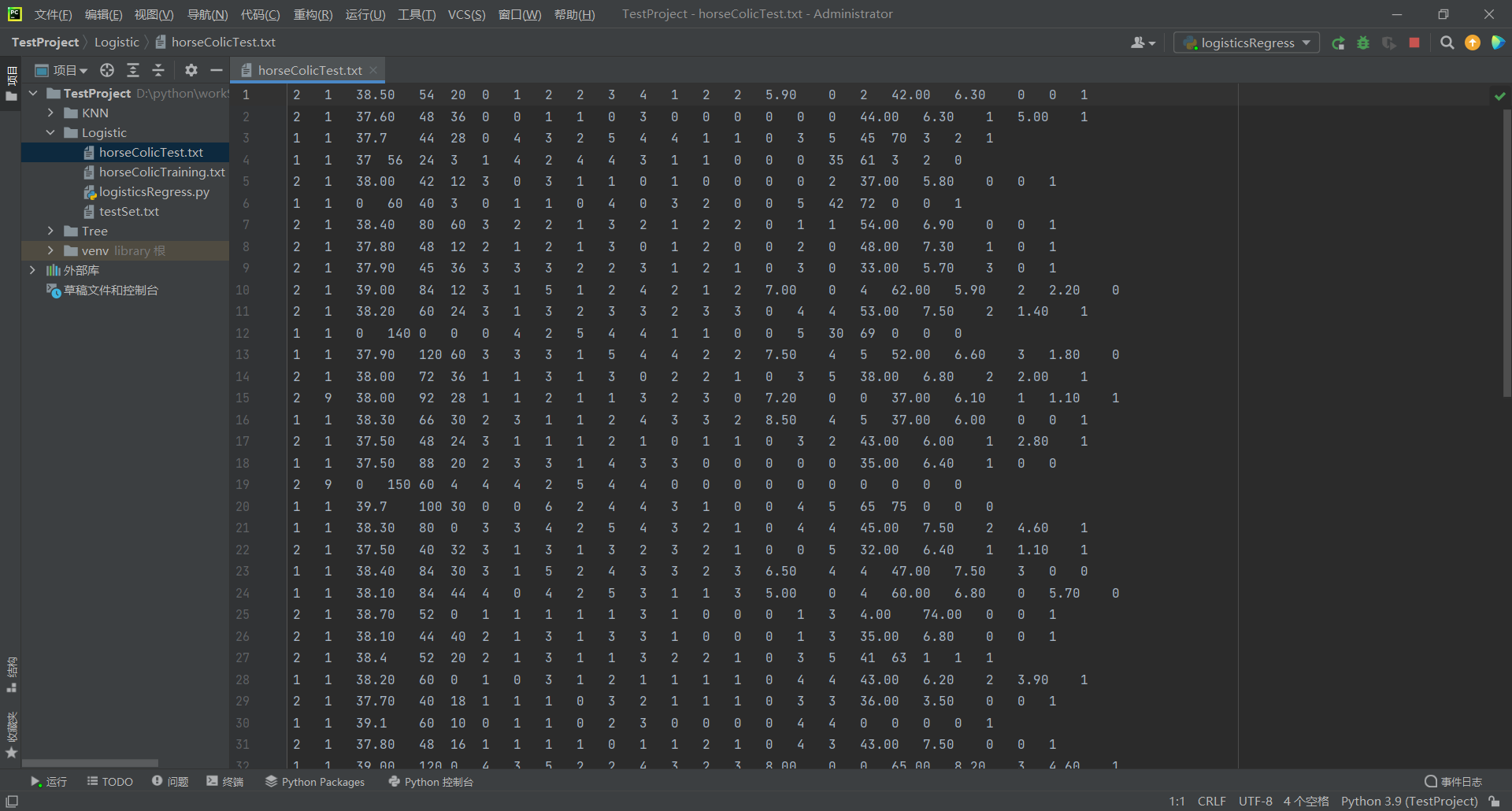
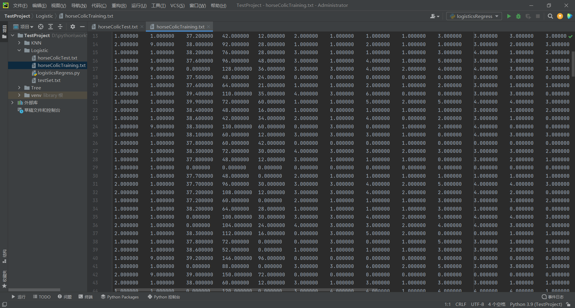
  The training data of the sick horse is stored in the text file as follows:

2. Test algorithm: use gradient rise algorithm for classification

# Classification function
def classifyVector(inX, weights):
    prob = sigmoid(sum(inX * weights))   # Calculate sigmoid value
    if prob > 0.5:                       # If the probability is greater than 0.5, the classification result of 1.0 is returned
        return 1.0
    else:                                # If the probability is less than or equal to 0.5, the classification result is returned as 0.0
        return 0.0

def colicTest1():
    # Read the test set and training set, and format the data
    frTrain = open('horseColicTraining.txt')      # Read training set file
    frTest = open('horseColicTest.txt')           # Read test set file
    trainingSet = []                              # Create data list
    trainingLabels = []                           # Create label list
    for line in frTrain.readlines():              # Read by line
        currLine = line.strip().split('\t')       # separate
        lineArr = []
        for i in range(21):
            lineArr.append(float(currLine[i]))
        trainingSet.append(lineArr)
        trainingLabels.append(float(currLine[21]))

    # Using improved random ascending gradient training
    trainWeights =  gradAscent(array(trainingSet), trainingLabels)
    errorCount = 0                                # Number of errors
    numTestVec = 0.0
    for line in frTest.readlines():               # Traverse each row of data
        numTestVec += 1.0                         # Number of test sets plus 1
        currLine = line.strip().split('\t')
        lineArr = []
        for i in range(21):
            lineArr.append(float(currLine[i]))
        if int(classifyVector(array(lineArr), trainWeights)) != int(currLine[21]):
            errorCount += 1                        # The prediction result is inconsistent with the true value, and the error number is increased by 1
    errorRate = (float(errorCount) / numTestVec)   # Calculation error rate
    print("The error rate of the test is: %f" % errorRate)
    return errorRate

# Average the results
def multiTest():
    numTests = 10
    errorSum = 0.0
    for k in range(numTests):
        errorSum += colicTest1()
    print("stay %d After iteration, the average error rate is: %f" % (numTests, errorSum / float(numTests)))

Test results: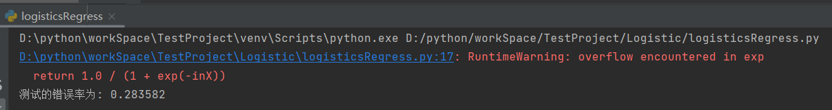  

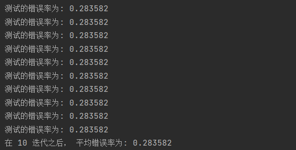
  As can be seen from the above results, the average error rate after 10 iterations is 28%.

3. Test algorithm: the improved random gradient rise algorithm is used for classification

         Using Logistic regression method for classification does not need to do much work. What needs to be done is to multiply each eigenvector on the test set by the regression coefficient obtained by the optimization method, sum the product results, and finally input them into the Sigmoid function. If the corresponding Sigmoid value is greater than 0.5, the prediction category label is 1, otherwise it is 0.

# Classification function
def classifyVector(inX, weights):
    prob = sigmoid(sum(inX * weights))   # Calculate sigmoid value
    if prob > 0.5:                       # If the probability is greater than 0.5, the classification result of 1.0 is returned
        return 1.0
    else:                                # If the probability is less than or equal to 0.5, the classification result is returned as 0.0
        return 0.0

#  Logistic classifier based on improved random gradient rise algorithm
def colicTest():
    # Read the test set and training set, and format the data
    frTrain = open('horseColicTraining.txt')      # Read training set file
    frTest = open('horseColicTest.txt')           # Read test set file
    trainingSet = []                              # Create data list
    trainingLabels = []                           # Create label list
    for line in frTrain.readlines():              # Read by line
        currLine = line.strip().split('\t')       # separate
        lineArr = []
        for i in range(21):
            lineArr.append(float(currLine[i]))
        trainingSet.append(lineArr)
        trainingLabels.append(float(currLine[21]))

    # Using improved random ascending gradient training
    trainWeights = stocGradAscent1(array(trainingSet), trainingLabels, 1000)
    errorCount = 0                                # Number of errors
    numTestVec = 0.0
    for line in frTest.readlines():               # Traverse each row of data
        numTestVec += 1.0                         # Number of test sets plus 1
        currLine = line.strip().split('\t')
        lineArr = []
        for i in range(21):
            lineArr.append(float(currLine[i]))
        if int(classifyVector(array(lineArr), trainWeights)) != int(currLine[21]):
            errorCount += 1                        # The prediction result is inconsistent with the true value, and the error number is increased by 1
    errorRate = (float(errorCount) / numTestVec)   # Calculation error rate
    print("The error rate of the test is: %f" % errorRate)
    return errorRate

# Average the results
def multiTest():
    numTests = 10
    errorSum = 0.0
    for k in range(numTests):
        errorSum += colicTest()
    print("stay %d After iteration, the average error rate is: %f" % (numTests, errorSum / float(numTests)))

Test results: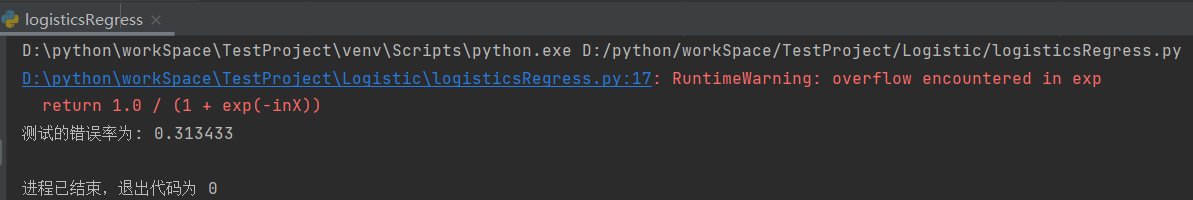

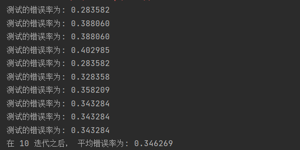
  As can be seen from the above results, the average error rate after 10 iterations is 34%.

4. Example: practice summary

Gradient rise algorithm: all samples participate in each update of regression coefficient.

• Advantages: accurate classification and global optimal solution
• Disadvantages: when there are many samples, the training speed is particularly slow
• Applicable occasions: data sets with few samples

Random gradient descent method: only one sample participates in each update of regression coefficient.

• Advantages: fast training
• Disadvantages: the accuracy will be reduced, not towards the overall optimal direction, and it is easy to obtain the local optimal solution
• Application: data sets with a large number of samples

      During this experiment, several small problems were encountered, such as the problem that the fitting curve was not displayed when drawing, and the problem of x and y dimensions was not noticed, resulting in being stuck in the drawing for half a day; In addition, it is easy to ignore the data types of variables, because python language has no strict requirements on defining variable types, and it is not written clearly like C or C + +, so I always forget to convert the data into lists or matrices, resulting in running errors in the process. In the end is to understand the experiment, do it, harvest a classification method, continue to work hard!!!