Pay attention to the public number [reverse communication ape] is more wonderful!!!
Check matrix H \boldsymbol{H} H

Definition of zero space:
H
\boldsymbol H
The zero space or kernel of H is written as
N
(
H
)
≜
{
x
∈
R
n
:
H
x
=
0
}
\mathcal{N}(\boldsymbol{H}) \triangleq\left\{\boldsymbol{x} \in \mathbb{R}^{n}: \boldsymbol{H} \boldsymbol{x}=\mathbf{0}\right\}
N(H)≜{x∈Rn:Hx=0}
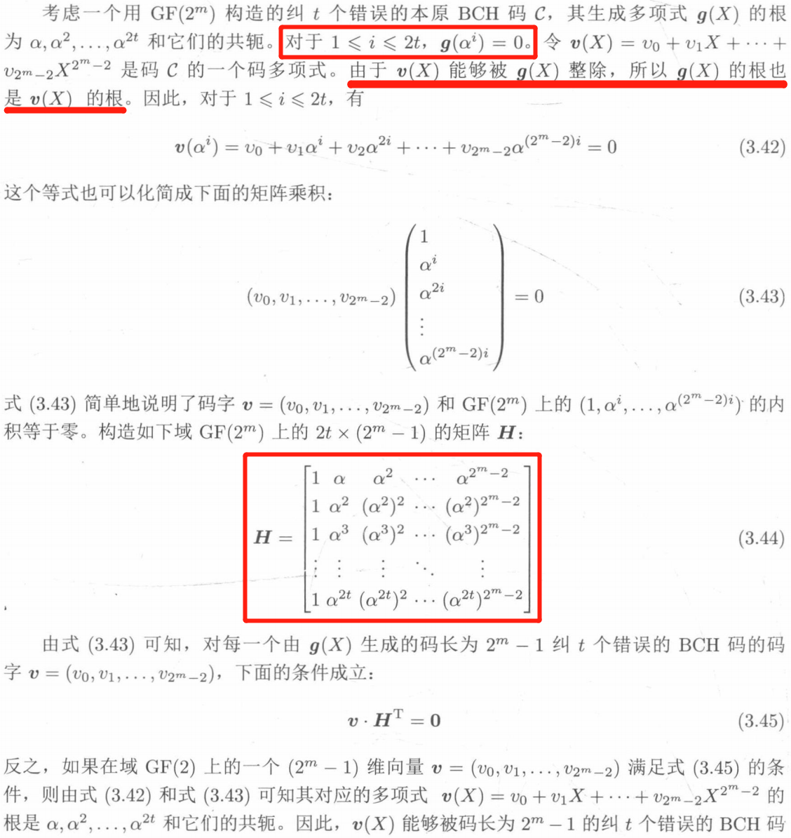
So, the BCH code space is H \boldsymbol H Zero space of H.
Decoding principle
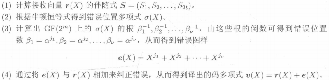
The specific principle derivation will not be repeated. Please refer to reference [1], and only its core idea is summarized here.
Decoding idea
1. Establishment of equations
According to adjoint
S
i
S_i
Si and wrong pattern
e
(
X
)
e(X)
Relationship of e(X)
S
i
=
e
(
α
i
)
S_i=\boldsymbol e(\alpha ^i)
Si=e(αi)
Get the wrong location
j
1
,
j
2
,
...
,
j
v
j_1,j_2,\ldots,j_v
j1, j2,..., jv
2
t
2t
2t adjoint relational equations:

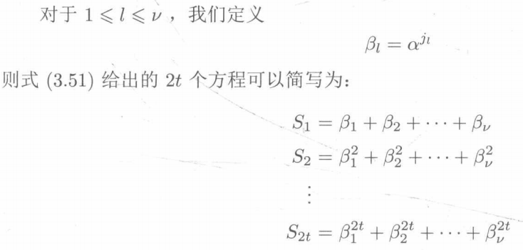
Solving the equations to get the error location can be used for error correction decoding. However, the equations are nonlinear and direct solution is not feasible, so the indirect solution method is adopted.
2 Newton identity
definition
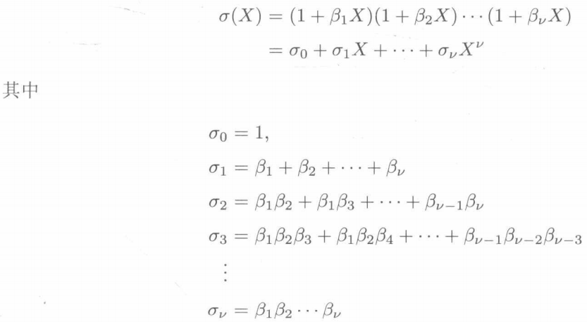
By observing the above formula, we can see that using the complete square expansion, this construction can connect the adjoint component with the coefficients of the wrong position polynomial to obtain the Newton identity
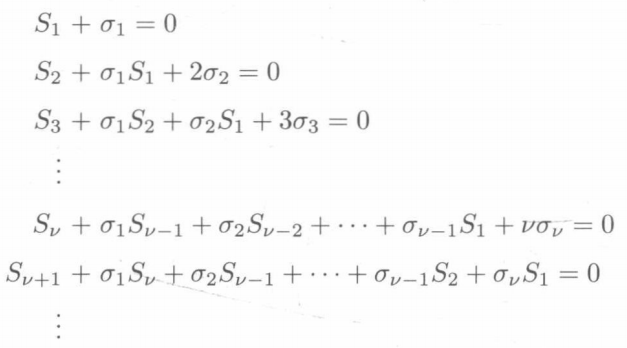
The error position polynomial is obtained by solving the equation with Newton identity
σ
(
X
)
\sigma(X)
σ (10) And its coefficient
σ
(
X
)
\sigma(X)
σ (10) And the reciprocal of the root is the wrong location. The decoding process is as follows.
3 decoding process
4 iterative solution of Newton identity (core of BM algorithm)
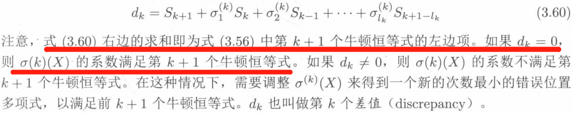
The Newton identity in decoding process (2) can be solved by Berlekamp Massey iterative algorithm (BM algorithm).
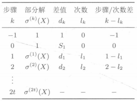
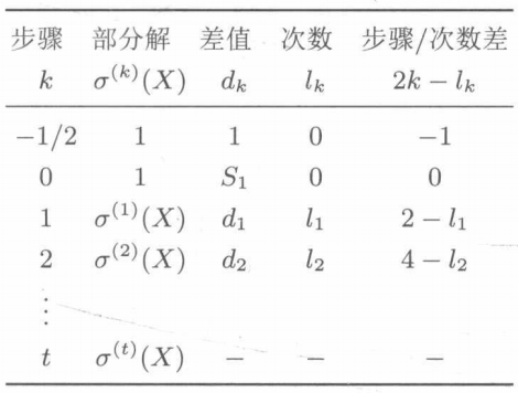
BM algorithm passed 2 t 2t The error position polynomial is solved by 2t iterations σ ( X ) \sigma(X) σ (10) , a bit like induction.
The first k k k times to get a minimum number of times σ ( k ) ( X ) \sigma^{(k)}(X) σ (k)(X), before meeting k k k equations. The first k + 1 k+1 k+1 times, based on σ ( k ) ( X ) \sigma^{(k)}(X) σ (k)(X) find the error position polynomial with the lowest degree next σ ( k + 1 ) ( X ) \sigma^{(k+1)}(X) σ (k+1)(X) to satisfy the previous k + 1 k+1 k+1 equations.
First, check
σ
(
k
)
(
X
)
\sigma^{(k)}(X)
σ (k) Whether the coefficient of (x) meets the requirements of paragraph
k
+
1
k+1
k+1 equations, if satisfied, then
σ
(
k
+
1
)
(
X
)
=
σ
(
k
)
(
X
)
\sigma^{(k+1)}(X)=\sigma^{(k)}(X)
σ(k+1)(X)=σ(k)(X)
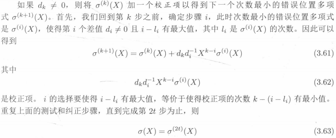
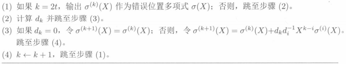
Otherwise, yes σ ( k ) ( X ) \sigma^{(k)}(X) σ (k)(X) obtained by adding correction items σ ( k + 1 ) ( X ) \sigma^{(k+1)}(X) σ (k+1)(X). The details are as follows:
calculation
Decoding algorithm description
q q Simplification of BM iterative algorithm for q-ary BCH Codes
Simplification of BM iterative algorithm for binary BCH Codes
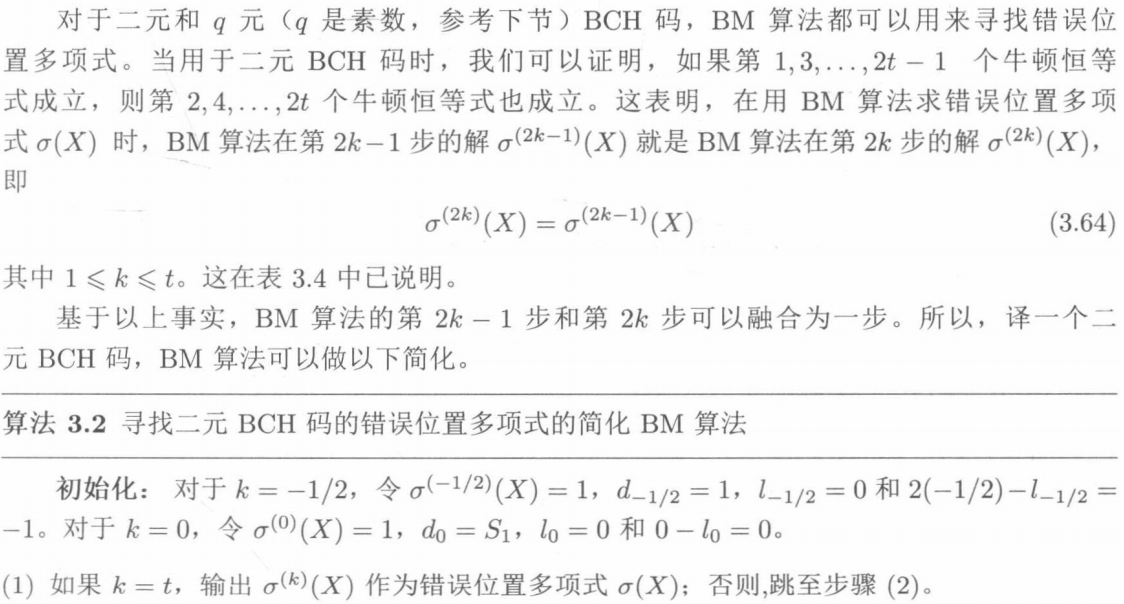
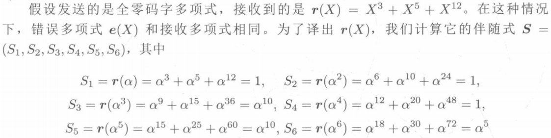
Restore BM iterative decoding process with an example
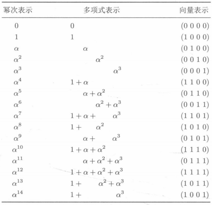
Taking (15,5,3)BCH code as an example, the code length is 15 and the error correction ability is good t = 3 t=3 t=3. The domain generating polynomial is p ( X ) = X 4 + X + 1 p(X)=X^4+X+1 p(X)=X4+X+1 (expressed as [1 0 1 1] by degree, expressed as 23 by octal number, hereinafter uniformly expressed as polynomial by octal), and the code generation polynomial is expressed as 2467 by octal number.
Generated domain
G
F
(
2
4
)
GF(2^4)
GF(24) is shown in the table below
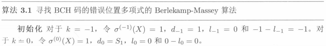
First initialize as follows
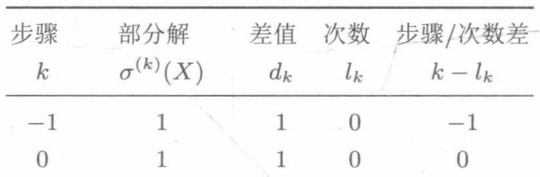
i
i
The initial value of i is - 1,
i
−
l
i
=
−
1
i-l_i=-1
i − li = − 1, start iteration:
①
k
=
1
k=1
When k=1, due to
d
0
=
1
≠
0
d_0=1\ne0
d0 = 1 = 0, so the calculated correction term is
d
0
d
−
1
−
1
X
0
−
(
−
1
)
σ
(
−
1
)
(
X
)
=
X
d_0d_{-1}^{-1}X^{0-(-1)}\sigma^{(-1)}(X)=X
d0d−1−1X0−(−1) σ (− 1)(X)=X, so
σ
(
1
)
(
X
)
=
1
+
X
\sigma^{(1)}(X)=1+X
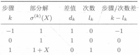
σ (1)(X)=1+X, from which
d
1
=
S
1
+
1
+
σ
1
(
1
)
S
1
=
S
2
+
1
⋅
S
1
=
0
d_1=S_{1+1}+\sigma_1^{(1)}S_1=S_2+1\cdot S_1=0
d1=S1+1+ σ 1 (1) S1 = S2 + 1 ⋅ S1 = 0, so
l
1
=
1
l_1=1
l1=1,
1
−
l
1
=
0
1-l_1=0
1−l1=0,
i
=
0
i=0
i=0,
i
−
l
i
=
0
i-l_i=0
i−li=0.
Update table to
②
k
=
2
k=2
When k=2, due to
d
1
=
0
d_1=0
d1 = 0, so
σ
(
2
)
(
X
)
=
σ
(
1
)
(
X
)
=
1
+
X
\sigma^{(2)}(X)=\sigma^{(1)}(X)=1+X
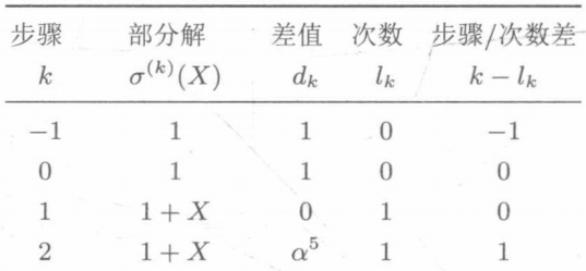
σ (2)(X)= σ (1)(X)=1+X, from which
d
2
=
S
2
+
1
+
σ
1
(
2
)
S
2
=
S
3
+
1
⋅
S
2
=
α
10
+
1
=
α
5
d_2=S_{2+1}+\sigma_1^{(2)}S_2=S_3+1\cdot S_2=\alpha^{10}+1=\alpha^5
d2=S2+1+ σ 1(2)S2=S3+1⋅S2= α 10+1= α 5, so
l
2
=
1
l_2=1
l2=1,
2
−
l
2
=
1
2-l_2=1
2−l2=1,
i
=
0
i=0
i=0,
i
−
l
i
=
0
i-l_i=0
i−li=0.
Update table to
③
k
=
3
k=3
When k=3, due to
d
2
=
α
5
≠
0
d_2=\alpha^5\ne0
d2= α 5 = 0, so the calculated correction term is
d
2
d
0
−
1
X
2
−
0
σ
(
0
)
(
X
)
=
α
5
X
2
d_2d_{0}^{-1}X^{2-0}\sigma^{(0)}(X)=\alpha^5X^2
d2d0−1X2−0 σ (0)(X)= α 5X2, so
σ
(
3
)
(
X
)
=
σ
(
2
)
(
X
)
+
α
5
X
2
σ
(
0
)
(
X
)
=
1
+
X
+
α
5
X
2
\sigma^{(3)}(X)=\sigma^{(2)}(X)+\alpha^5X^2\sigma^{(0)}(X)=1+X+\alpha^5X^2
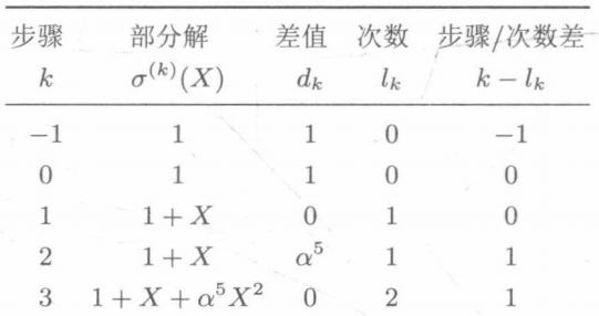
σ (3)(X)= σ (2)(X)+ α 5X2 σ (0)(X)=1+X+ α 5x2, resulting in
d
3
=
S
3
+
1
+
σ
1
(
3
)
S
3
+
σ
2
(
3
)
S
2
=
S
4
+
1
⋅
S
3
+
α
5
S
2
=
1
+
α
10
+
α
5
=
0
d_3=S_{3+1}+\sigma_1^{(3)}S_3+\sigma_2^{(3)}S_2=S_4+1\cdot S_3+\alpha^5S_2=1+\alpha^{10}+\alpha^5=0
d3=S3+1+ σ 1(3)S3+ σ 2(3)S2=S4+1⋅S3+ α 5S2=1+ α 10+ α 5 = 0, so
l
3
=
2
l_3=2
l3=2,
3
−
l
3
=
1
3-l_3=1
3−l3=1,
i
=
2
i=2
i=2,
i
−
l
i
=
1
i-l_i=1
i−li=1.
Update table to
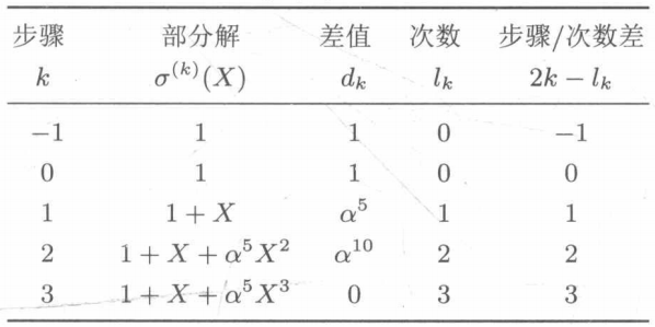
④ And so on, and finally
2
t
2t
The results of 2t iterations are as follows:
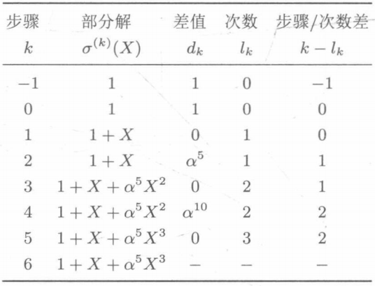
The result of the simplified BM algorithm is:
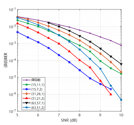
Simulation performance and analysis
simulation result
Main program code
File name: bch_codec.m
clear; close all; clc

%% (15,11,1) BCH code
% px=[1 0 0 1 1];  % 23 Primitive polynomial
% p = length(px)-1;
% [a,a_dec,log_a] = sub_gf_gen( px ); % Finite field
% gx=[1 0 0 1 1]; % 23
% t=1;

%% (15,7,2) BCH code
% gx=[1 1 1 0 1 0 0 0 1]; % 721
% t=2;

%% (31,26,1) BCH code
% px=[1 0 0 1 0 1];  % 45
% p = length(px)-1;
% [a,a_dec,log_a] = sub_gf_gen( px ); % Finite field
% gx=[1 0 0 1 0 1]; % 45
% t=1;
%% (31,21,2) BCH code
% gx=[1 1 1 0 1 1 0 1 0 0 1]; % 3551
% t=2;

%% (63,57,1) BCH code
px=[1 0 0 0 0 1 1];  % 103
p = length(px)-1;
[a,a_dec,log_a] = sub_gf_gen( px ); % Finite field
% gx=[1 0 0 0 0 1 1]; % 103
% t=1;

%% (63,51,2) BCH code
gx=[1 0 1 0 1 0 0 1 1 1 0 0 1]; % 12471
t=2;

m = length(px)-1;
n=2^m-1; % Code length
pg = length(gx) -1; % Generating polynomial degree
k=n-pg; % Information chief

codnum = 100000;
snr = 5:0.5:10;
snrlen = length(snr);
num_bef = zeros(1,snrlen);
num_aft = zeros(1,snrlen);
tic
parfor i = 1:snrlen
    SNRi = snr(i);
    for j = 1:codnum
%         rng('shuffle');
        u = randi([0,1],1,k);
        v = sub_encod_bch(u,gx,0);
        vn = awgn(1-2*v,SNRi,'measured');
        r = double(vn<0);
        num_bef(i) = num_bef(i)+biterr(r,v);
        [rdec,pos_err,flag]=sub_decod_bch(r,t,a,log_a,p);
        num_aft(i) = num_aft(i)+biterr(rdec,v);
    end
    disp(['Signal to noise ratio ',num2str(SNRi),' complete']);
end
toc
ber_bef = num_bef/n/codnum;
ber_aft = num_aft/n/codnum;
Drawing code
File name: plot_bch_dec.m
clear; clc; close all;

snr=5:0.5:10;
len = length(snr);
lw = 2;

%% Bit error rate before decoding
load('ber_bef.mat');
figure;semilogy(snr,ber_bef,'Marker','x','color',[0.49 0.18 0.56],'LineWidth',lw);hold on;

%% (15,11,1)BCH code
load('ber_aft_bch_15_11_1.mat');
semilogy(snr,ber_aft,'Marker','s','color',[0 161/255 59/255],'LineWidth',2);hold on;

%% (15,7,2)BCH code
load('ber_aft_bch_15_7_2.mat');
semilogy(snr,ber_aft,'o-b','LineWidth',lw);hold on;

%% (31,26,1)BCH code
load('ber_aft_bch_31_26_1.mat');
semilogy(snr,ber_aft,'Marker','d','color',[0.85 0.33 0.10],'LineWidth',lw);hold on;

%% (31,21,2)BCH code
load('ber_aft_bch_31_21_2.mat');
semilogy(snr,ber_aft,'^-r','LineWidth',lw);hold on;

%% (63,57,1)BCH code
load('ber_aft_bch_63_57_1.mat');
semilogy(snr(4:end),ber_aft(4:end),'Marker','v','color',[0 0 0],'LineWidth',lw);hold on;

%% (63,51,2)BCH code
load('ber_aft_bch_63_51_2.mat');
semilogy(snr,ber_aft,'Marker','p','color',[0 0.4470 0.7410],'LineWidth',lw);hold on;

xlabel('SNR (dB)');ylabel('decoding BER'); grid on;
legend('Before decoding','(15,11,1)','(15,7,2)','(31,26,1)','(31,21,2)','(63,57,1)','(63,51,2)');
set(gca,'FontSize',13,'Fontname', 'Microsoft YaHei ');
Partial subroutine code
Finite field multiplication subroutine
File name: sub_gf_mul.m
function [ z ] = sub_gf_mul( x, y, n )
% Galois field element multiplication, parameter meaning:
%% input:
% x y: Represents the power of two elements and the value range-inf or[0,n-1]
% n: 2^m-1

%% output:
% z: Represents the power of the product

if x>=0 && y>=0
    z = mod(x+y,n);
else
    z=-inf;
end
Finite field addition subroutine
File name: sub_gf_add.m
function [ z ] = sub_gf_add( x, y, a, log_a )
% Galois domain element addition, parameter meaning:
%% input:
% x y: Represents the power of two elements and the value range-inf or[0,n-1]
% n: 2^m-1

%% output:
% z: Represents the power of the sum of two elements. When the sum is 0, the power is specified as-inf,Convenient calculation

if x<0
    z=y;
elseif y<0
    z=x;
elseif x==y
    z=-inf;
else
    sum=mod(a(x+1,:)+a(y+1,:),2);
    sum_deci = bi2de(sum, 'left-msb');
    z = log_a(sum_deci);
end
All code downloads
| file name | function |
|---|---|
| bch_codec.m | main program |
| sub_gf_gen.m | Finite field generation subroutine |
| sub_gf_add.m | Finite field addition subroutine |
| sub_gf_mul.m | Finite field multiplication subroutine |
| sub_poly_div.m | Polynomial division subroutine |
| sub_encod_bch.m | BCH coding subroutine |
| sub_decod_bch.m | Simplified BM iterative decoding subroutine for BCH code |
| plot_bch_dec.m | Drawing subroutine |
| ber_aft_bch_15_7_2.mat | (15,7,2) code decoding error rate data file |
| ber_aft_bch_15_11_1.mat | (15,11,1) code decoding error rate data file |
| ber_aft_bch_31_26_1.mat | (31,26,1) code decoding error rate data file |
| ber_aft_bch_31_21_2.mat | (31,21,2) code decoding error rate data file |
| ber_aft_bch_63_57_1.mat | (63,57,1) code decoding error rate data file |
| ber_aft_bch_63_51_2.mat | (63,51,2) code decoding error rate data file |
a) Local tyrant, please feel free
Directly click the following link to download all codes (with comments) and drawing data from the blogger's resources
All code downloads: https://download.csdn.net/download/wlwdecs_dn/45111931
You can also subscribe Channel coding column , refer to the detailed explanation of each subroutine
The principle of generating finite field by primitive polynomial and its MATLAB implementation
Principle of binary polynomial division circuit and its implementation in MATLAB
b) Good people who support bloggers, please look at this
Pay attention to the public number [reverse communication], password: BCH, which can be obtained by simply supporting one wave
c) White whoring party
nothing
reference
[1]William E Ryan, Shu Lin. channel coding: classic and modern [M]. Electronic Industry Press, 2017