Video link: The final collection of PyTorch deep learning practice_ Beep beep beep_ bilibili

This secondary implementation is a more complex neural network. Although the model looks very complex, in order to reduce code redundancy and improve code reusability, we can define the neural network with the same structure as a class to improve code reusability and make the code more concise.

The neural network result diagram we want to realize is shown in the figure below:

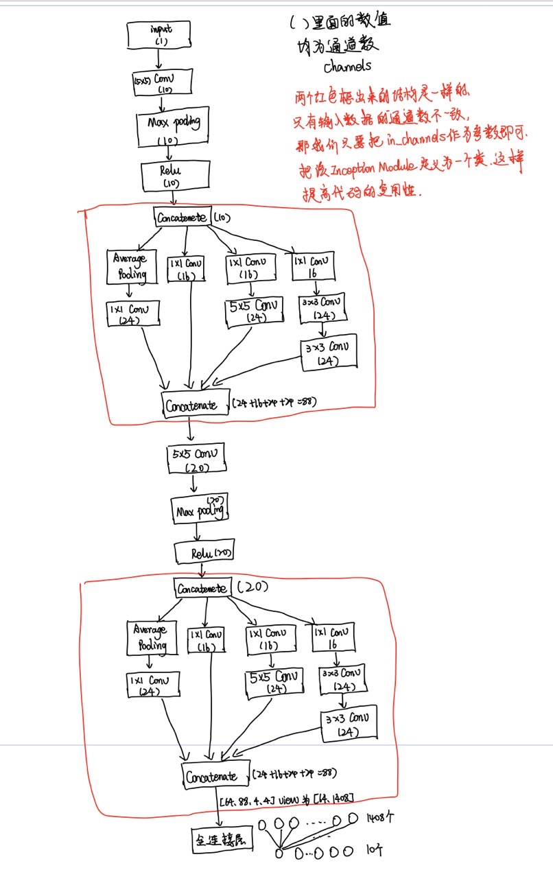
  If you understand the above picture, it's easy to write code now. I'll explain the model class that implements Inception Modele first. First of all, because we need to connect the number of channels on the four shunts later, no matter what, batch other than the number of channels_ Size, width and height cannot be changed. Therefore, when the inception model implements the convolution operation, we have filled it, that is, the width and height after each convolution remain unchanged. It is very important to understand here.

Note: padding=2 means that 2 pixels are added around the original image.

Let's take a look at the code implementation of Inception Modele (that is, the neural network structure model I drew in red above):

Left 1: refers to the first neural network forward propagation route on the left of Inception Modele

import numpy as np
from torchvision.datasets import MNIST
from torchvision import transforms
from torch.utils.data import DataLoader
import torch
import torch.nn.functional as F
import matplotlib.pyplot as plt


# Inception Module
class InceptionA(torch.nn.Module):
    # Batch required_ Size, width and height cannot be changed, otherwise they cannot be spliced. Only channels can be changed
    def __init__(self, in_channels):
        super(InceptionA, self).__init__()
        # Generation layer
        # On the left, the pool layer is in forward
        self.branch_pool = torch.nn.Conv2d(in_channels, 24, kernel_size=1)
        
        # Left two
        self.branch1x1 = torch.nn.Conv2d(in_channels, 16, kernel_size=1)
        
        # Left three
        self.branch5x5_1 = torch.nn.Conv2d(in_channels, 16, kernel_size=1)
        self.branch5x5_2 = torch.nn.Conv2d(16, 24, kernel_size=5, padding=2)
        
        # Left four
        self.branch3x3_1 = torch.nn.Conv2d(in_channels, 16, kernel_size=1)
        self.branch3x3_2 = torch.nn.Conv2d(16, 24, kernel_size=3, padding=1)
        self.branch3x3_3 = torch.nn.Conv2d(24, 24, kernel_size=3, padding=1)

    def forward(self, x):
        # Forward propagation
        # Left one
        # Pool layer, average
        branch_pool = F.avg_pool2d(x, kernel_size=3, padding=1, stride=1)
        branch_pool = self.branch_pool(branch_pool)

        # Left two
        branch1x1 = self.branch1x1(x)

        # Left three
        branch5x5 = self.branch5x5_2(self.branch5x5_1(x))

        # Left four
        branch3x3 = self.branch3x3_3(self.branch3x3_2(self.branch3x3_1(x)))
        
        # connect
        outputs = [branch_pool, branch1x1, branch5x5, branch3x3]
        return torch.cat(outputs, dim=1)  # Number of channels = 24 + 24 + 24 + 16 = 88

Next, the implementation class code of the whole model is given:

# Whole neural network
class Net(torch.nn.Module):
    def __init__(self):
        super(Net, self).__init__()
        self.conv1 = torch.nn.Conv2d(1, 10, kernel_size=5)
        self.conv2 = torch.nn.Conv2d(88, 20, kernel_size=5)

        self.incep1 = InceptionA(in_channels=10)
        self.incep2 = InceptionA(in_channels=20)

        self.mp = torch.nn.MaxPool2d(2)
        # Last full connection layer
        self.fc = torch.nn.Linear(1408, 10)  # 88*4*4

    def forward(self, x):
        in_size = x.size(0)
        x = F.relu(self.mp(self.conv1(x)))
        x = self.incep1(x)
        x = F.relu(self.mp(self.conv2(x)))
        x = self.incep2(x)  # torch.Size([64, 88, 4, 4])
        # print(x.size())  # First output the values of each order, and then determine the shape of the full connection layer torch.Size([64, 88, 4, 4]). Here, determine self.fc = nn.Linear(1408, 10)
        # Enter the full connection layer and convert to level 2 [batch_size,C*H*W]
        x = x.view(in_size, -1)
        x = self.fc(x)
        return x

Well, the above two parts are a little difficult. In fact, it is not too difficult to write the implementation class according to the neural network structure diagram I drew. The other parts are the same as the previous job code.

The following is the full code implementation:

import numpy as np
from torchvision.datasets import MNIST
from torchvision import transforms
from torch.utils.data import DataLoader
import torch
import torch.nn.functional as F
import matplotlib.pyplot as plt


# Internal neural network
class InceptionA(torch.nn.Module):
    # Batch required_ Size, width and height cannot be changed, otherwise they cannot be spliced. Only channels can be changed
    def __init__(self, in_channels):
        super(InceptionA, self).__init__()
        # Generate convolution
        self.branch_pool = torch.nn.Conv2d(in_channels, 24, kernel_size=1)

        self.branch1x1 = torch.nn.Conv2d(in_channels, 16, kernel_size=1)

        self.branch5x5_1 = torch.nn.Conv2d(in_channels, 16, kernel_size=1)
        self.branch5x5_2 = torch.nn.Conv2d(16, 24, kernel_size=5, padding=2)

        self.branch3x3_1 = torch.nn.Conv2d(in_channels, 16, kernel_size=1)
        self.branch3x3_2 = torch.nn.Conv2d(16, 24, kernel_size=3, padding=1)
        self.branch3x3_3 = torch.nn.Conv2d(24, 24, kernel_size=3, padding=1)

    def forward(self, x):
        # first floor
        # Pool layer, average
        branch_pool = F.avg_pool2d(x, kernel_size=3, padding=1, stride=1)
        branch_pool = self.branch_pool(branch_pool)

        # The second floor
        branch1x1 = self.branch1x1(x)

        # Third floor
        branch5x5 = self.branch5x5_2(self.branch5x5_1(x))

        # Fourth floor
        branch3x3 = self.branch3x3_3(self.branch3x3_2(self.branch3x3_1(x)))

        outputs = [branch_pool, branch1x1, branch5x5, branch3x3]
        return torch.cat(outputs, dim=1)  # Number of channels = 24 + 24 + 24 + 16 = 88


# Whole neural network
class Net(torch.nn.Module):
    def __init__(self):
        super(Net, self).__init__()
        self.conv1 = torch.nn.Conv2d(1, 10, kernel_size=5)
        self.conv2 = torch.nn.Conv2d(88, 20, kernel_size=5)

        self.incep1 = InceptionA(in_channels=10)
        self.incep2 = InceptionA(in_channels=20)

        self.mp = torch.nn.MaxPool2d(2)
        # Last full connection layer
        self.fc = torch.nn.Linear(1408, 10)  # 88*4*4

    def forward(self, x):
        in_size = x.size(0)
        x = F.relu(self.mp(self.conv1(x)))
        x = self.incep1(x)
        x = F.relu(self.mp(self.conv2(x)))
        x = self.incep2(x)  # torch.Size([64, 88, 4, 4])
        # print(x.size())  # First output the values of each order, and then determine the shape of the full connection layer torch.Size([64, 88, 4, 4]). Here, determine self.fc = nn.Linear(1408, 10)
        # Enter the full connection layer and convert to level 2 [batch_size,C*H*W]
        x = x.view(in_size, -1)
        x = self.fc(x)
        return x


# Load dataset
# 1. Prepare dataset
# Processing data
transform = transforms.Compose([
    transforms.ToTensor(),
    transforms.Normalize((0.1307,), (0.3081,))
])
batch_size = 64
# Training set
mnist_train = MNIST(root='../dataset/mnist', train=True, transform=transform, download=True)
train_loader = DataLoader(dataset=mnist_train, shuffle=True, batch_size=batch_size)
# Test set
mnist_test = MNIST(root='../dataset/mnist', train=False, transform=transform, download=True)
test_loader = DataLoader(dataset=mnist_test, shuffle=True, batch_size=batch_size)

model = Net()
# 3. Construct loss function and optimizer
criterion = torch.nn.CrossEntropyLoss()
optimizer = torch.optim.SGD(model.parameters(), lr=0.01, momentum=0.5)


# 4. Training and testing
# Define training method, a training cycle
def train(epoch):
    running_loss = 0.0
    for idx, (inputs, target) in enumerate(train_loader, 0):
        # The code here is no different from before
        # Forward
        y_pred = model(inputs)
        loss = criterion(y_pred, target)
        # reverse
        optimizer.zero_grad()
        loss.backward()
        # to update
        optimizer.step()

        running_loss += loss.item()
        if idx % 300 == 299:  # The average loss per 300 prints is% 299 instead of 300 because idx starts from 0
            print(f'epoch={epoch + 1},batch_idx={idx + 1},loss={running_loss / 300}')
            running_loss = 0.0


# Accuracy list for drawing
accuracy_list = []


# One test cycle
def test():
    # Number of samples with correct predictions
    correct_num = 0
    # Number of all samples
    total = 0
    # When testing, we do not need to calculate the gradient, so we can add this sentence without gradient tracking
    with torch.no_grad():
        for images, labels in test_loader:
            # Get predicted value
            outputs = model(images)
            # Gets the location of the maximum value of dim=1, which represents the predicted tag value
            _, predicted = torch.max(outputs.data, dim=1)
            # Accumulate the number of samples in each batch to obtain the number of all samples in a test cycle
            total += labels.size(0)
            # Accumulate the predicted correct samples of each batch to obtain all the predicted correct samples of a test cycle
            correct_num += (predicted == labels).sum().item()
        print(f'Accuracy on test set:{100 * correct_num / total}%')  # Print the accuracy of a test cycle
        accuracy_list.append(100*correct_num / total)


if __name__ == '__main__':
    # Test the number of neurons in the whole connection layer
    # for idx, (inputs, target) in enumerate(train_loader, 0):
    #     model(inputs)
    #     break
    # The training cycle is 10 times. The number of samples of all training sets is trained and tested each time
    for epoch in range(10):
        train(epoch)
        test()
    # Drawing
    plt.plot(np.arange(10),accuracy_list)
    plt.xlabel('epoch')
    plt.ylabel('accuracy %')
    plt.show()

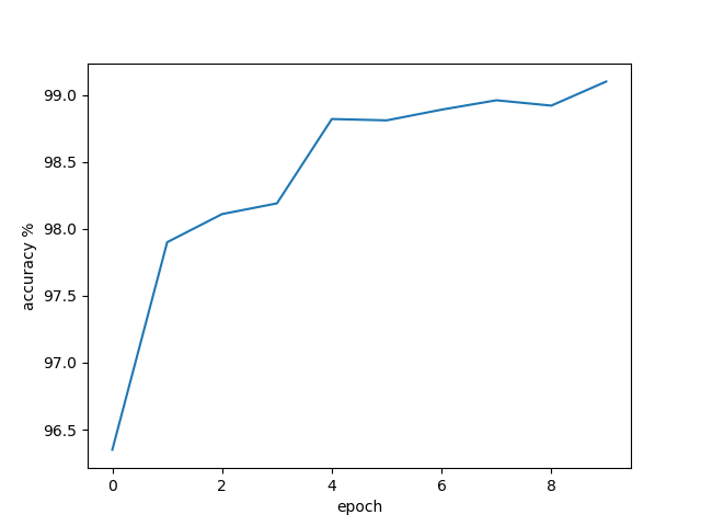
The results are as follows:

epoch=1,batch_idx=300,loss=0.9408395903557539
epoch=1,batch_idx=600,loss=0.19775621948142846
epoch=1,batch_idx=900,loss=0.1403631071994702
Accuracy on test set:96.35%

.......

epoch=9,batch_idx=300,loss=0.03314510397089179
epoch=9,batch_idx=600,loss=0.03342989099541834
epoch=9,batch_idx=900,loss=0.03618314559746068
Accuracy on test set:98.92%
epoch=10,batch_idx=300,loss=0.029011620228023578
epoch=10,batch_idx=600,loss=0.03060439710029944
epoch=10,batch_idx=900,loss=0.03674590568523854
Accuracy on test set:99.1%

  Well, if you have any questions, please point them out. Thank you