Hello, everyone. Today I'd like to share with you the logical regression algorithm in python machine learning. The main contents include:
(1) Algorithm principle; (2) Accuracy and recall; (3) Case application -- cancer case prediction.
At the end of the paper, there are data sets and complete python code
1. Concept understanding
Logistic regression, or LR for short, is characterized by the ability to convert our feature input set into probabilities of 0 and 1. Generally speaking, regression is not used in classification, but logical regression can perform well in binary classification (i.e. divided into two types of problems).
Logistic regression is essentially linear regression, but a layer of Sigmod function mapping is added to the mapping from feature to result, that is, sum the feature lines first, and then use Sigmoid function to solve the most hypothetical function by probability, and then classify.
The Sigmoid function is: 
sigmoid function is shaped like s curve, the lower side is infinitely close to 0 and the upper side is infinitely close to 1
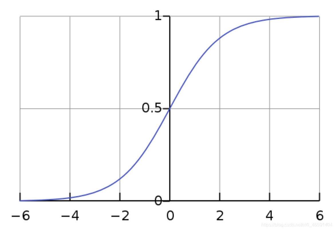
For example, in the process of prediction, if the prediction result is greater than 0.5, we think it belongs to class I, and if it is less than 0.5, we think it belongs to class II, and then we realize class II Classification.
Advantages: it is suitable for scenes where a classification probability needs to be obtained. It is simple and fast
Disadvantages: it can only be used to deal with two classification problems, and it is difficult to deal with multi classification problems
Application: Whether it is sick, financial fraud, false account number, etc
2. Accuracy and recall
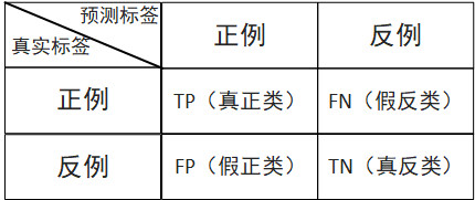
As shown in the following table, if I predict that a person has cancer, his real value is also cancer, then this situation is called TP real case; If I predict that a person has cancer and his real value is no cancer, this situation is called FN false counterexample.
(1) Accuracy rate: the prediction result is the proportion of positive samples that are truly positive (used to indicate whether it is accurate or not)
The formula is: 
Among 100 people, my prediction is that 20 people have cancer. Among the 20 people, only 5 really had cancer and 15 did not. Then the accuracy is P=5/(5+15)=0.25
(2) Recall rate: the proportion of samples with positive prediction results (indicating the completeness of the investigation and the ability to distinguish between positive samples)
The formula is: 
Example: now there are 20 people with cancer. Among these people, I have detected that 18 people have cancer and 2 people have not detected it. The recall rate is R=18/(18+2)
(3) Comprehensive indicators: sometimes there are contradictions between P and R indicators, so they need to be considered comprehensively. The most common method is F-Measure.
The formula is: 
If F1 is large, the comprehensive performance is better
Import method: from sklearn.metrics import classification_report
classification_report() Function parameters
y_true: 1-dimensional array, or label indicator array / sparse matrix, true value.
y_pred: 1-dimensional array, or label indicator array / sparse matrix, predicted value
Labels: list, shape = [n_labels], an optional list of label indexes contained in the report.
target_names: list of strings, optional display names matching the labels (in the same order)
sample_weight: an array similar to shape = [n_samples], optional, sample weight
Digits: int, the number of digits of the output floating-point value
3. Case application - cancer case prediction
3.1 Sklearn implementation
Logistic regression method import: from sklearn.linear_model import LogisticRegression
Parameter setting: Reference blog https://blog.csdn.net/jark_/article/details/78342644
Penalty: penalty item, str type. The optional parameters are l1 and l2. The default is l2. Specifies the specification used in the penalty item.
L1 specification assumes that the parameters of the model meet the Laplace distribution, and L2 assumes that the model parameters meet the Gaussian distribution. The so-called normal form is to add constraints on parameters so that the model will not over fit. In theory, with constraints, we should be able to obtain results with stronger generalization ability.
Dual: dual or primitive method, bool type, False by default. The dual method is only used to solve the L2 penalty term of linear multi-core. When the number of samples > sample characteristics, dual is usually set to False.
tol: the standard to stop solving, float type, the default is 1e-4. Is to stop when the solution reaches how much, and think that the optimal solution has been found.
C: Regularization coefficient λ The reciprocal of, float type, defaults to 1.0. Must be a positive floating point number. Like SVM, smaller values represent stronger regularization.
fit_intercept: whether there is intercept or deviation. bool type. The default is True.
intercept_scaling: only when the regularization item is "liblinear" and fit_ Useful when intercept is set to True. float type, the default is 1.
class_weight: used to indicate various types of weights in the classification model. It can be a dictionary or 'balanced' string. It is not entered by default, that is, no weight is considered, that is, None.
If you choose to enter, you can choose balanced to let the class library calculate the type weight by itself, or enter the weight of each type by itself. For example, for the binary model of 0,1, we can define class_weight={0:0.9,1:0.1}, so the weight of type 0 is 90%, and the weight of type 1 is 10%. If class_weight if balanced is selected, the class library will calculate the weight according to the training sample size. The larger the sample size of a certain type, the lower the weight. The smaller the sample size, the higher the weight. When class_ When the weight is balanced, the class weight is calculated as follows: n_samples / (n_classes * np.bincount(y)). n_samples is the number of samples, n_ Classes is the number of classes. Np.bincount (y) will output the number of samples of each class. For example, y=[1,0,0,1,1], then np.bincount(y)=[2,3].
random_state: random number seed, int type, optional parameter. The default is none. It is only useful when the regularization optimization algorithm is sag and liblinear.
solver: select parameters for the optimization algorithm. There are only five optional parameters, namely Newton CG, lbfgs, liblinear, sag and saga. The default is liblinear.
solver parameter determines our optimization method for logistic regression loss function. There are four algorithms to choose from, namely:
Liblinear: it is implemented using the open source liblinear library and internally uses the coordinate axis descent method to iteratively optimize the loss function.
lbfgs: a kind of quasi Newton method, which uses the second derivative matrix of loss function, i.e. Hessian matrix, to iteratively optimize the loss function.
Newton CG: a kind of Newton method, which uses the second derivative matrix of loss function, namely Hessian matrix, to iteratively optimize the loss function.
sag: random average gradient descent, which is a variant of the gradient descent method. The difference from the ordinary gradient descent method is that only a part of the samples are used to calculate the gradient in each iteration, which is suitable for the case of large sample data.
saga: linear convergent stochastic optimization algorithm with variable weight.
Verbose: log verbose length, int type. The default is 0. That is, the training process is not output. When 1, the results are occasionally output. If it is greater than 1, it is output for each sub model.
warm_start: hot start parameter, bool type. The default is False. If True, the next training is in the form of an additional tree (reuse the previous call as initialization).
3.1 cancer prediction
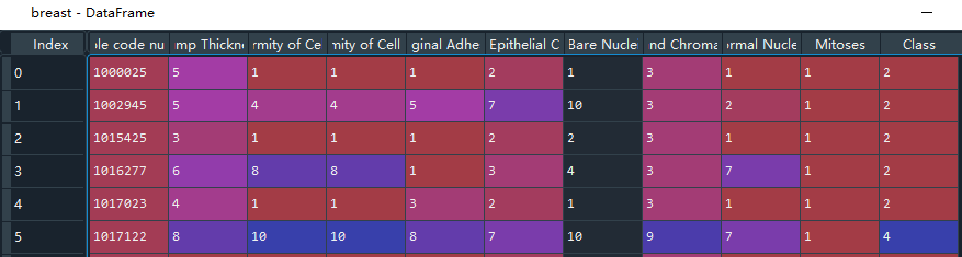
The data set contains 10 eigenvalue data and 1 target data, with the character '?' Represents missing data, and the number 2 in the target represents benign cancer and 4 represents malignant cancer.
Data set download address: https://archive.ics.uci.edu/ml/machine-learning-databases/breast-cancer-wisconsin/
Names stores the column index name of each item of data. When pandas imports the dataset, the first row of data will be regarded as the data index name by default, while the original data has no column index name. We need to customize the column pd.read_ CSV (file path, names = column name)
#(1) Data acquisition
import pandas as pd
import numpy as np
# Cancer data path
filepath = 'C:\\Users\\admin\\.spyder-py3\\test\\File processing\\cancer\\breast-cancer-wisconsin.data'
# Each characteristic name of cancer
names = ['Sample code number', 'Clump Thickness', 'Uniformity of Cell Size', 'Uniformity of Cell Shape','Marginal Adhesion', 'Single Epithelial Cell Size', 'Bare Nuclei', 'Bland Chromatin','Normal Nucleoli', 'Mitoses', 'Class']
# The first row is not used as the column index name by default, and the column index name is customized
breast = pd.read_csv(filepath,names=names)
# Check the unique value. The Class column represents whether the has cancer. Use the. unique() function to check the different values in this column
unique = breast['Class'].unique()  #There are only two cases, which are two classification problems. 2 represents benign and 4 represents malignant
3.2 data processing
First pass . info() Function to check whether there are missing data nan and duplicate data in the data, not in this example. Then the character '?' For processing, first set '?' Convert to nan value, and then use the. dropna() function to delete the line where nan is located. After completion, divide the eigenvalue and target value. Then divide the training set and test set, and the test set takes 25% of the data.
#(2) Data processing
breast.info()  #Check for missing values and duplicate data
# String type data '?' exists in this dataset
# Will '?' Convert to nan
breast = breast.replace(to_replace='?',value=np.nan)
# Delete the row where nan is located
breast = breast.dropna()

# Eigenvalues are all data except the class column
features = breast.drop('Class',axis=1)
# The target value is the class column
targets = breast['Class']

#(3) Divide training set and test set
from sklearn.model_selection import train_test_split
x_train,x_test,y_train,y_test = train_test_split(features,targets,test_size=0.25)
3.3 standardized treatment
Because different units and too large data span will affect the accuracy of the model, the eigenvalues of training data and test data are standardized. The specific methods of feature engineering will be introduced in the following chapters, which will be understood here first.
#(4) Characteristic Engineering
# Import standardization method
from sklearn.preprocessing import StandardScaler
# Receiving standardization method
transfer = StandardScaler()
# Eigenvalue x for training_ Train extracts features and normalizes them
x_train = transfer.fit_transform(x_train)
# Eigenvalue x for test_ Test standardization
x_test = transfer.transform(x_test)
3.4 logistic regression prediction
Since the results in the cancer data are only 2 and 4, benign and malignant, which belong to the dichotomy problem, the logistic regression method can be used to predict. Here, in order to facilitate your understanding, the logistic regression method with default parameters is adopted. The. fit() function receives the eigenvalues and target values required by the training model, the prediction function. predict() receives the eigenvalues required for prediction, and the scoring method. score() calculates the accuracy through the real results and prediction results. The accuracy of the model is 0.97
#(5) Logistic regression prediction
# Import logistic regression method
from sklearn.linear_model import LogisticRegression
# Receiving logistic regression method
logist = LogisticRegression()
# penalty=l2 regularization; tol=0.001, stop when the loss function is less than; C=1 penalty term. The smaller the penalty, the smaller the penalty, which is one third of the multiplication strength of ridge regression
# train
logist.fit(x_train,y_train)
# forecast
y_predict = logist.predict(x_test)
# Calculation accuracy of scoring method
accuracy = logist.score(x_test,y_test)
3.5 accuracy and recall
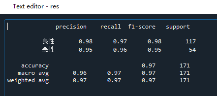
#(6) Accuracy and recall
# Import
from sklearn.metrics import classification_report
# classification_report()
# Parameters (real value, predicted value, labels=None,target_names=None)
# labels: name each item in the class column, such as 2 and 4 of the question
# target_names: name

# Calculate accuracy and recall
res = classification_report(y_test,y_predict,labels=[2,4],target_names=['Benign','malignant'])
precision means accuracy; Recall indicates the recall rate; F1 score represents comprehensive index; support represents the predicted number of people. The recall rate of this model is 0.97 for benign and 0.96 for malignant; This example is to detect cancer. We hope to find all people with cancer. Even if they are not cancer, they can also be further examined. Therefore, we need a model with high recall rate.
Dataset acquisition:
Index of /ml/machine-learning-databases/breast-cancer-wisconsin
Full code:
#(1) Data acquisition
import pandas as pd
import numpy as np
# Cancer data path
filepath = 'C:\\Users\\admin\\.spyder-py3\\test\\File processing\\cancer\\breast-cancer-wisconsin.data'
# Each characteristic name of cancer
names = ['Sample code number', 'Clump Thickness', 'Uniformity of Cell Size', 'Uniformity of Cell Shape','Marginal Adhesion', 'Single Epithelial Cell Size', 'Bare Nuclei', 'Bland Chromatin','Normal Nucleoli', 'Mitoses', 'Class']
# The first row is not used as the column index name by default, and the column index name is customized
breast = pd.read_csv(filepath,names=names)
# Check the unique value. The Class column represents whether the has cancer. Use the. unique() function to check the different values in this column
unique = breast['Class'].unique()  #There are only two cases, which are two classification problems. 2 represents benign and 4 represents malignant

#(2) Data processing
breast.info()  #Check for missing values and duplicate data
# String type data '?' exists in this dataset
# Will '?' Convert to nan
breast = breast.replace(to_replace='?',value=np.nan)
# Delete the row where nan is located
breast = breast.dropna()

# Eigenvalues are all data except the class column
features = breast.drop('Class',axis=1)
# The target value is the class column
targets = breast['Class']

#(3) Divide training set and test set
from sklearn.model_selection import train_test_split
x_train,x_test,y_train,y_test = train_test_split(features,targets,test_size=0.25)

#(4) Characteristic Engineering
# Import standardization method
from sklearn.preprocessing import StandardScaler
# Receiving standardization method
transfer = StandardScaler()
# Eigenvalue x for training_ Train extracts features and normalizes them
x_train = transfer.fit_transform(x_train)
# Eigenvalue x for test_ Test standardization
x_test = transfer.transform(x_test)


#(5) Logistic regression prediction
# Import logistic regression method
from sklearn.linear_model import LogisticRegression
# Receiving logistic regression method
logist = LogisticRegression()
# penalty=l2 regularization; tol=0.001, stop when the loss function is less than; C=1 penalty term. The smaller the penalty, the smaller the penalty, which is one third of the multiplication strength of ridge regression
# train
logist.fit(x_train,y_train)
# forecast
y_predict = logist.predict(x_test)
# Calculation accuracy of scoring method
accuracy = logist.score(x_test,y_test)


#(6) Accuracy and recall
# Import
from sklearn.metrics import classification_report
# classification_report()
# Parameters (real value, predicted value, labels=None,target_names=None)
# labels: name each item in the class column, such as 2 and 4 of the question
# target_names: name

# Calculate accuracy and recall
res = classification_report(y_test,y_predict,labels=[2,4],target_names=['Benign','malignant'])
# precision accuracy; Recall recall rate; Comprehensive index F1 score; support: predicted number of people