Note: This is a machine learning practical project (with data + code). If you need data + complete code, you can get it directly at the end of the article.

1. Project background
For the fault diagnosis of semiconductor etcher, it is necessary to collect and obtain the data of the etching process of semiconductor etcher, analyze and process the data. The original data of the semiconductor etcher in this paper comes from the operation state data of LAM9600 plasma etcher when processing wafers. This paper mainly introduces the pre-processing of etching process data of semiconductor etcher, mainly including the following contents: analysis of semiconductor etcher data, performance characteristics of semiconductor etcher fault data and extraction of abnormal data, and then extraction and data integration of semiconductor etcher fault data. Through data preprocessing, the fault data set with unified dimension is obtained, which lays a foundation for the later classification design and experimental verification of test data set.
Wafer depth feature representation in semiconductor manufacturing process is the premise and basis of wafer data anomaly detection. This paper studies how to use the deep learning theory to design the deep neural network architecture. From the unmarked original wafer data, unsupervised autonomous learning can characterize the health state characteristics, and then establish the baseline model through the health characteristics to identify the fault state data set.
2. Data collection
The data sets are as follows:
Training dataset: etch_train.csv
Test dataset: etch_test.csv
Data fields include: Run ID, Time, etc
In practical application, you can replace it according to your own data.
Characteristic data: data other than this data item TCP Rfl Pwr
Tag data: TCP Rfl Pwr
3. Data preprocessing
)Fault analysis of semiconductor etcher
As one of the important basic equipment in semiconductor manufacturing, semiconductor etching machine has a direct impact on its working performance, manufacturing quality and production efficiency. When there is a fault in the semiconductor etcher, relevant technicians shall timely find and correctly deal with the equipment points where the fault data occurs, so as to ensure the safety of the operation of the etching equipment and reduce the impact on the operation of the etching equipment due to the fault.
In order to study the data-driven anomaly detection method in the etching process, a variety of different faults are introduced in the experimental etching process, including the artificial changes of gas flow and chuck pressure, a total of 20 types. In other words, these 20 different physical quantities may cause abnormalities of etching equipment, and 20 data changes identified in this fault type will cause the final fault of the whole data. The data collected this time includes 19 variables collected from the sensor, 1 time variable and 2 process variables, a total of 22 variables. Each variable is a column, which constitutes the training and test data. The specific name of each variable and its corresponding meaning are shown in the table below.
Data header description
| Serial number | Listing | Data meaning |
| 1 | Run ID | Unit serial number |
| 2 | Time | time |
| 3 | Step Number | Manufacturing process steps |
| 4 | BCl3 Flow | Process physical quantity |
| 5 | Cl2 Flow | |
| 6 | RF Btm Pwr | |
| 7 | RF Btm Rfl Pwr | |
| 8 | Endpt A | |
| 9 | He Press | |
| 10 | Pressure | |
| 11 | RF Tuner | |
| 12 | RF Load | |
| 13 | RF Phase Err | |
| 14 | RF Pwr | |
| 15 | RF Impedance | |
| 16 | TCP Tuner | |
| 17 | TCP Phase Err | |
| 18 | TCP Impedance | |
| 19 | TCP Top Pwr | |
| 20 | TCP Rfl Pwr | |
| 21 | TCP Load | |
| 22 | Vat Valve |
)Data analysis of semiconductor etcher
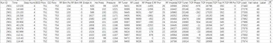
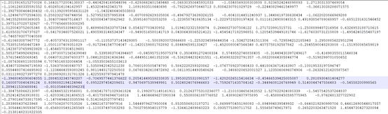
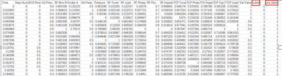
The original data of the semiconductor etcher in this paper comes from some data of the operation state of LAM 9600 plasma etcher. The collected data provided shall be stored in the form of CSV file, and the data generated in the production process of etching equipment shall be collected and stored in the table in each unit. As shown in the figure.
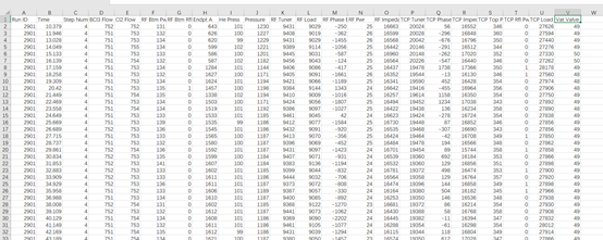
Raw training data
Taking the first row of data as an example, it represents the physical quantities of each process of the fourth process step of the wafer No. 2901 at time point 10.379. Nearly 50 pieces of data were collected in each step of each wafer, and a total of 85 wafers were collected in the training data set. A total of 7608 pieces of data. The same test data set collects the physical quantity data of 31 wafers in etching process steps 4 and 5, with a total of 5162 data.
)Fault data extraction of semiconductor etcher
The purpose of this section is to extract abnormal data, i.e. fault data, from training data set and test data set, so as to prepare for subsequent data analysis and neural network reading. In semiconductor etcher data, fault data can be regarded as abnormal fluctuation data compared with normal data, that is, data with large error. At present, the most commonly used statistical methods for screening error data are Dixon criterion, panta criterion, Grubbs criterion, Chauvenet criterion, etc. each of these methods has its own advantages and disadvantages. When the sample size of the data is greater than or equal to 50 (the sample size used in this paper has been greater than 50), we choose reinda criterion to eliminate the large error data in the sample data, which is the best choice and will get a better effect. Therefore, this paper adopts the reinda criterion.
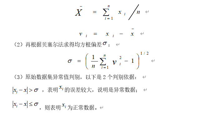
In this paper, the rheinda criterion is used to extract the fault data in the semiconductor etching data according to a certain criterion range after calculating the average value and root mean square deviation of the data of the same dimension. After calculating the average value and root mean square deviation, we can use the reinda criterion to confirm the abnormal data in the semiconductor etching data according to the two important parameters of average value and root mean square deviation. The reinda code is also known as 3 σ The criterion is a common and easy to learn outlier judgment and elimination method. It is judged according to the difference between the sample data and the calculated mean and root mean square deviation. The specific calculation method is as follows:

As shown in the figure, taking the data of the test data set wafer 2915 as an example, calculate the arithmetic mean, residual error and root mean square error of each variable data, extract the fault data in the semiconductor etching data according to the two parameters of mean value and root mean square deviation, and extract the fault data in the data set.
As shown in the figure, in the Pressure column, the mean value is 1232.537, the root mean square deviation is 18.645, and the value is 0.7924, The value of is about 0.5, 0.7924 > 0.5, so it is determined that the physical quantity BCl3 Flow data 1309, 1303, 1303, 1295 and 1296 of the wafer 2915 in step 5 belong to abnormal data.
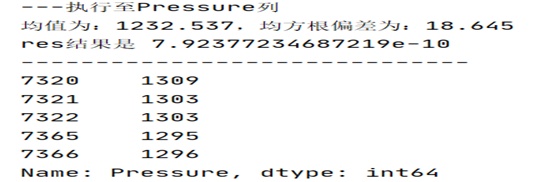
Abnormal data in the Pressure column
In the Pressure column shown, the value is 0.44, The value of is about 0.5, but 0.44 < 0.5, so it is determined that the wafer 2915 belongs to normal data.
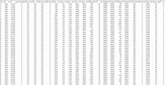
For the analysis of the experimental data, the test data set containing fault data is divided into two parts according to the ratio of 7:3, which are named done data set and done data set respectively_ Test data set, set the fault tag as 0 and 1, 0 represents no fault and 1 represents fault. Through the reinda criterion, we can make a judgment with abnormal value data, and mark the fault tag at the end of the data. The figure is a screenshot of bad data values extracted from done dataset, as shown in the figure:
Bad data value of etcher
4) Data integration
After fault extraction, there are great differences in the dimension of data. Whether using neural network, deep learning or other AI Artificial intelligence algorithms, most algorithm models can not deal with the data dimension well. Therefore, we need a method to realize an adaptive dimensionality reduction process, which removes the dimensions that have little impact on the data analysis results, but will not affect the data analysis results.
Through the analysis of process physical quantities with large data differences, we set the data fault label as 0 and 1, where 0 represents no fault and 1 represents fault. Therefore, we can eliminate the physical process quantities RF Btm Rfl Pwr and TCP Rf1 Pwr as data difference items, because their data difference is between 0 and 1, and the fault tag is also 0 and 1, which will affect the network reading judgment, so they are eliminated. When reading the training data, Run ID, Time and Step Number will not be input into the training network as data dimension, Because their changes are fixed, there are 17 physical quantities finally input into the network, so the input dimension of the network is 17.
After fault extraction and data integration, the fault data set of network training is sorted out. On the basis of fault data and normal data set, the dimension is integrated, and a certain number of data sets with fault data are added to the original training data set. The integrated data set is used as the sample data set for neural network training, and the sample data is marked. At this time, the data are marked as two types, namely 0 and 1. As shown in the figure:
Key code display:
 data_0 = pd.read_csv('etch_test.csv')  # Read data
    data_0.drop(['RF Btm Rfl Pwr', 'TCP Rfl Pwr'], axis=1, inplace=True)  # Remove RF Btm Rfl Pwr TCP Rfl Pwr exception column value
    labellist = np.zeros(len(data_0['Run ID']))  # Generate 0 filled array
    results = []  # Define an empty list
    data = data_0.groupby('Run ID')  # Group by Run ID
    for key in set(data_0['Run ID'].tolist()):  # The Run ID column is de duplicated and then cycled
        data_1 = data.get_group(key)  # grouping
        ColNames = data_1.columns.tolist()  # Get all column names
        print('---Execute to' + str(key) + 'number')  # Print execution log
        for j in ColNames:  # Circular column name
            df = data_1[j]  # Gets the specified column data
            ks_res = JisuanJun(df)  # Call JisuanJun calculation function
            result = Suanfa(df, ks_res)  # Call Suanfa calculation function
            # none and empty in series
            if result is not None and result.empty == False:  # Null values are different from NONE
                # series key value pair direct items
                results.append(result.items())  # Key value pair pairing

    for i in results:  # Cycle all result data
        for key, value in i:  # Form key value pairs
            labellist[key + 2] = 1  # Tag data assignment
    data_0['Label'] = labellist  # Assign tag data to data_0 list
    min_max_scaler = preprocessing.MinMaxScaler()  # Define normalization function
    # Standardized training set data
    for key in set(data_0['Run ID'].tolist()):  # The Run ID column is de duplicated and then cycled
        data_1 = data.get_group(key)  # grouping
        ColNames = data_1.columns.tolist()  # Get all column names
        print('---Execute to' + str(key) + 'number')  # Print execution log
        for j in ColNames:  # Circular column name
            df = data_1[j]  # Gets the specified column data
            _range = np.max(df) - np.min(df)  # Calculate the maximum minus the minimum for each column
            data_train_nomal = (df - np.min(df)) / _range  # Start normalizing data
            data_1[j] = data_train_nomal  # Normalized data assignment
    data_1.to_csv(r"test000.csv", mode='a', index=False)  # Save standardized data
4. Construction of fault diagnosis model of semiconductor etcher based on RBF neural network
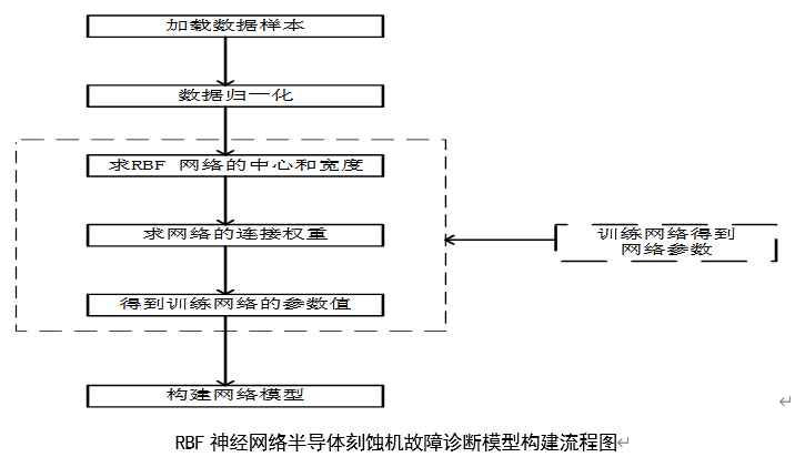
1) Model overview
Through the study of relevant learning algorithms and the basic structure of RBF neural network, it is known that the following problems need to be considered in order to preliminarily build an RBF neural network model:
(1) Determining the number of input layer nodes of RBF neural network is equivalent to the input dimension of samples;
(2) Determine the parameters of the hidden layer, including data center, width and the number of hidden layer nodes.
(3) The number of neurons in the output layer of RBF neural network and the interconnected weights of hidden layer nodes and output layer nodes are determined.
For the first problem, the data set has been obtained in Chapter 3. The data are 17 dimensions. Therefore, the input layer node of RBF neural network is set to 17 and normalized. As shown in the figure below, the flow chart of constructing the fault diagnosis model of semiconductor etcher based on RBF neural network is shown.
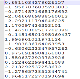
)Input layer data normalization
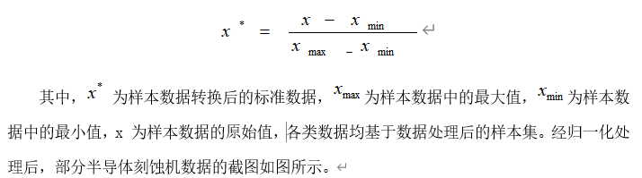
Data normalization is to limit all data to a certain range and reduce the data value after processing the data by some algorithm or function. The advantages of normalization processing are: on the one hand, it can reduce the large gap between data; On the other hand, it can also ensure that the convergence speed of the program is accelerated. For the training of RBF neural network, it will indirectly affect the accuracy of the training network. In this paper, the fast and simple linear normalization conversion principle is adopted to directly set the limit range and limit the sample data value to the range (- 1, 1). The specific formula is as follows:
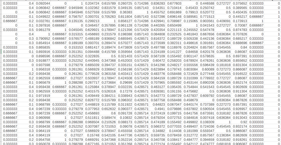
Partial data after normalization
In this way, after removing the number, time and process steps that have little impact on the experimental results, we can set the input dimension of the input layer of RBF neural network to 17, and then the training network can directly read the normalized samples. Here, we separate the test data set by 7:3, of which 70% is used for the experimental verification and comparison of the network, 30% is used for abnormal data detection of the network.
3) RBF neuron activation function
Each RBF neuron calculates the similarity between the input and its prototype vector (obtained from the training set). An input vector more similar to the prototype returns a result closer to 1. The choice of similar functions may be different, but the most popular is based on Gaussian model. The following is a Gaussian equation with one-dimensional input.
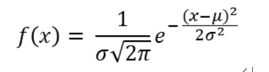
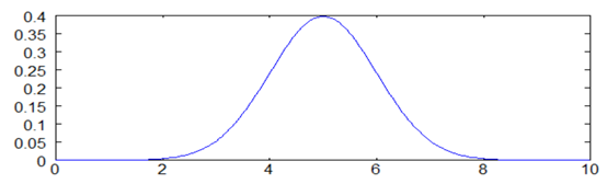
Where x is the input, Mu is the average, and sigma is the standard deviation. This will produce the familiar bell curve shown below, with its center on the average mu (in the figure below, the average is 5 and sigma is 1).
The activation function of RBF neurons is slightly different, which is usually written as:
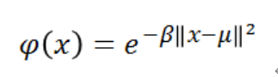
In the Gaussian distribution, mu represents the mean value of the distribution. Here, it is the prototype vector, which is located at the center of the bell curve. For the activation function phi, we are not directly interested in the value of standard deviation sigma, so we make some simplified modifications.
The first change is that we delete the external coefficient 1 / (sigma * sqrt (2 * pi)). This term usually controls the height of Gauss. However, here, the weight applied by the output node is redundant. During training, the output node will learn the correct coefficients or "weights" to apply to the neuron's response. The second change is that we replace the internal coefficient 1 / (2 * sigma ^ 2) with a single parameter "beta". Should β The coefficient controls the width of the bell curve. Similarly, in this case, we don't care about the value of sigma, we just care about whether there is a coefficient controlling the width of the bell curve. Therefore, we simplify the equation by replacing the term with a single variable.
4) The activation of RBF neurons can produce different beta values
When we apply the equation to an n-dimensional vector, the expression of the symbol also changes slightly. The parallel bars in the activation equation indicate that we are the Euclidean distance between X and Mu and square the result. For one-dimensional Gaussian, this is simplified to (x-mu) ^ 2.
It is important to note that the basic measure used here to evaluate the similarity between the input vector and the prototype is the Euclidean distance between the two vectors.
Similarly, when the input is equal to the prototype vector, each RBF neuron will produce the maximum response. This allows it to be used as a measure of similarity and sum the results of all RBF neurons.
When we move out of the prototype vector, the response decreases exponentially. It can be recalled from the RBFN architecture description that the output nodes of each category adopt the weighted sum of each RBF neuron in the network. In other words, each neuron in the network will have a certain impact on the classification decision. However, the exponential decline of the activation function means that the neurons whose prototypes are far away from the input vector actually make little contribution to the results.
)Parameter design of hidden layer node
The network hidden layer parameters mainly include three important parameters: the center of radial basis function, the number and width of hidden layer nodes. In the K-means algorithm, the setting of the number of clusters K is interdependent with the number of hidden layer nodes. The clustering category K is the number of hidden layer nodes in the network model.
The basic idea of K-means algorithm: for the data sample set, the data in the sample set is divided into k classes by determining the distance between samples. In this k category, we can choose to take the larger proportion of each of the 17 variables as the normal value, try to minimize the distance between samples in each category, and let the normal data gather together as a category. The naturally abnormal data are located outside the community, and make the distance between K categories as large as possible, The distance shall be as large as possible in order to make it easier for the network to identify normal data and abnormal data.
The basic steps of K-means algorithm are as follows:
(1) From the input sample data, K objects are randomly selected as the starting clustering center. In the initial stage, K is naturally 17;
(2) Calculate the distance from each data object to each cluster center. Here, the distance formula between two points on the coordinate is directly used, and it is classified into the nearest cluster according to the calculation results. The data value is classified into which category is closest to which category;
(3) Recalculate the center of each cluster;
(4) Repeat steps ② and ③ until the center of clustering does not change or is less than a set threshold, indicating that the algorithm is over.
After training, the maximum distance between the final centers of the network is 238.328, which is between the dimensions Bcl3 Flow and Rf After the distance between the clustering centers of Phase Err is calculated by k-means algorithm, the width of the network is further determined. The solution formula is:
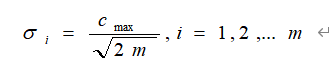
m represents the number of training samples, Is the maximum distance between the selected centers. Finally, the network width is determined to be 2. Through the continuous iteration of network training and data convergence, the number of neurons in the network can be 600. The central value of the network is written based on python program, which is not used as the return value. It is equivalent to that the values of various parameters are not uniquely determined, but determined based on the best effect of network training.
)Output layer design
The parameter setting of the output layer mainly includes the connection weight value between the hidden layer and the output layer (the RBF neural network implementation based on python does not return the weight value) and the number of nodes in the output layer. In this paper, there are 17 types of semiconductor etcher faults, corresponding to 17 types of data in the data set.
The last set of parameters is the output weight. Gradient descent (also known as least mean square) can be used for training. Firstly, for each data point in the training set, the activation value of RBF neurons is calculated. These activation values become the training input of gradient descent. The linear equation requires a bias term, so we always add the fixed value "1" to the beginning of the activation value vector. Gradient descent must be run separately for each output node (that is, for each class in the dataset). For output labels, use the value "1" for samples belonging to the same category as the output node and "0" for all other samples. For example, if our dataset has three categories and we are learning the weights of output node 3, all category 3 examples should be marked "1" and all category 1 and 2 examples should be marked 0.
After the center, width and weight of RBF neural network are determined, the output results of the network model are trained, as shown in Figure 4.3. Each row in the figure represents the normalized output result of the selected data.
center value

Network delta value
Network weight value
Key code display:
def load_data(file_name): # Define function
    # Get the feature and label data, and then return it in matrix form
    file = open(file_name)  # Open file
    feature_data = []  # Define an empty list of features
    label0 = []  # Define an empty list of tags
    for line in file.readlines(): # Cycle through each row of data
        feature_tmp = [] # Define a temporal list
        lines = line.strip().split("\t") # Split data with spaces
        for i in range(len(lines) - 1):
            data = float(lines[i]) / 1000  # Divide each row by 1000
            feature_tmp.append(data) # The processed data is added to the temporary list
        label0.append(int(lines[-1])) # The processed data is added to the label list
        feature_data.append(feature_tmp) # The processed data is added to the feature list
    file.close()  # Close file
    n_output = 1  # Definition n_output is Changshu 1

    return mat(feature_data), mat(label0).transpose(), n_output   # Output feature and label data in matrix form


def hanshu(x): # Define function

    return x   # Realize the return of the neuron activation function of the output layer


def hidden_out(feature, center, delta):  # Define function
    '''
    realization rbf Function (hidden layer neuron output function)
    input:feature(mat):Data characteristics
          center(mat):rbf Function center
          delta(mat): rbf Function extension constant
   Last hidden layer output
    '''
    m, n = shape(feature)  # Gets the shape of the feature
    m1, n1 = shape(center)  # Gets the shape of the center of the rbf function
    hidden_out = mat(zeros((m, m1)))  # Get hidden layer output
    for i in range(m):  # Cyclic characteristic data
        for j in range(m1): # Circular rbf function center data
            hidden_out[i, j] = exp(-1.0 * (feature[i, :] - center[j, :]) * (feature[i, :] - center[j, :]).T / (
                    2 * delta[0, j] * delta[0, j]))   # Hidden layer function calculation
    return hidden_out   # Hidden layer calculation output


def predict_in(hidden_out, w): # Define prediction function
    '''
    Calculate the input of the output layer
    input:  hidden_out(mat):Output of hidden layer
            w1(mat):Weight from hidden layer to output layer
            b1(mat):Offset from hidden layer to output layer
    output: predict_in(mat):Input of output layer
    '''
    m = shape(hidden_out)[0]  # Get hidden layer shape
    print('Get hidden layer shape')
    print(m)
    predict_in = hidden_out * w  # Hidden layer multiplied by weight
    return predict_in   # Return results


def predict_out(predict_in):  # Define function
    '''Output of output layer
    input:  predict_in(mat):Input of output layer
    output: result(mat):Output of output layer
    '''
    n = len(predict_in)  # Get predict_ Length in
    result = hanshu(predict_in) # Call hanshu function for calculation
    result[0:n // 4] = 1 # result assignment
    result[n // 4: :] = 0.084 # result assignment
    return result   # Return results

def predict_test(predict_in): # Define function
    '''Output of test data output layer
    input:  predict_in(mat):Input of output layer
    output: result(mat):Output of output layer
    '''
    n = len(predict_in)  # Get predict_ Length in
    result = hanshu(predict_in) # Call hanshu function for calculation
    result[0:n // 4] = 1 # result assignment
    result[n // 4: Assignment] = 0 # result:
    return result   # Return results


def rbf_train(feature, label, n_hidden, maxCycle, alpha, n_output): # Define training function
    '''
    Calculate the input of the hidden layer
    input:  feature(mat):features
            label(mat):label
            n_hidden(int):Number of hidden layer nodes
            maxCycle(int):Maximum number of iterations
            alpha(float):Learning rate
            n_output(int):Number of nodes in the output layer
    output: center(mat):rbf Function center
            delta(mat):rbf Function extension constant
            w(mat):Weight from hidden layer to output layer
    '''
    m, n = shape(feature)  # Get feature shape
    # Initialize function center, weight and function extension constant
    center = mat(random.rand(n_hidden, n))  # rbf function converts the central data into matrix form
    center = center * (8.0 * sqrt(6) / sqrt(n + n_hidden)) - mat(ones((n_hidden, n))) * (
            4.0 * sqrt(6) / sqrt(n + n_hidden))  # Initialize rbf function center
    delta = mat(random.rand(1, n_hidden)) # Transforming rbf function expansion constant into matrix form
    delta = delta * (8.0 * sqrt(6) / sqrt(n + n_hidden)) - mat(ones((1, n_hidden))) * (
            4.0 * sqrt(6) / sqrt(n + n_hidden)) #  Initialize rbf function extension constant
    w = mat(random.rand(n_hidden, n_output)) # The weights from the hidden layer to the output layer are converted into matrix form
    w = w * (8.0 * sqrt(6) / sqrt(n_hidden + n_output)) - mat(ones((n_hidden, n_output))) * (
            4.0 * sqrt(6) / sqrt(n_hidden + n_output)) # Initializes the weight from the hidden layer to the output layer

    # train
    iter = 0 #Define initialization iteration
    while iter <= maxCycle: # Increase the judgment. If the number of iterations is greater than maxCycle, stop the cycle
        # Signal forward propagation
        hidden_output = hidden_out(feature, center, delta) # Call hidden_ The out function calculates the output of the hidden layer

        output_in = predict_in(hidden_output, w)  # Call predict_in function to calculate the input of the output layer

        output_out = predict_out(output_in)  # Call predict_ The out function calculates the output of the output layer

        # Back propagation of error
        error = mat(label - output_out) # Calculate reverse error
        for j in range(n_hidden): # Loop hidden layer
            sum1 = 0.0 # Define initialization value
            sum2 = 0.0 # Define initialization value
            sum3 = 0.0 # Define initialization value
            for i in range(m):  # Cyclic characteristic data
                sum1 += error[i, :] * exp(
                    -1.0 * (feature[i] - center[j]) * (feature[i] - center[j]).T / (2 * delta[0, j] * delta[0, j])) * (
                                feature[i] - center[j]) # Calculate the rbf function center for preliminary calculation
                sum2 += error[i, :] * exp(
                    -1.0 * (feature[i] - center[j]) * (feature[i] - center[j]).T / (2 * delta[0, j] * delta[0, j])) * (
                                feature[i] - center[j]) * (feature[i] - center[j]).T  # Calculate the expansion constant of rbf function and make a preliminary calculation
                sum3 += error[i, :] * exp(
                    -1.0 * (feature[i] - center[j]) * (feature[i] - center[j]).T / (2 * delta[0, j] * delta[0, j])) # Calculate the weight from the hidden layer to the output layer
            delta_center = (w[j, :] / (delta[0, j] * delta[0, j])) * sum1  # Calculate the rbf function center for the final calculation
            delta_delta = (w[j, :] / (delta[0, j] * delta[0, j] * delta[0, j])) * sum2 # Calculate the expansion constant of rbf function for final calculation
            delta_w = sum3  # Weight assignment
            # Modified weights and rbf function center and extension constants
            center[j, :] = center[j, :] + alpha * delta_center  # Modified rbf function center
            delta[0, j] = delta[0, j] + alpha * delta_delta # Modified rbf expansion constant
            w[j, :] = w[j, :] + alpha * delta_w #  Fixed weight from hidden layer to output layer
        if iter % 10 == 0:  # Make iterative judgment
            cost = (1.0 / 2) * get_loss(get_predict(feature, center, delta, w) - label)  # Call get_loss function for loss calculation
            print("\t-------- iter: ", iter, " ,cost: ", cost) # Print loss calculation log
        if cost < 15:  #  Stop the stack if the loss function value is less than 15
            break
        iter += 1
    return center, delta, w  # Returns the rbf function center, the rbf extension constant, and the weight from the hidden layer to the output layer


def get_loss(cost):  # Define loss function
    '''
    Calculates the value of the current loss function
    input:  cost(mat):Difference between predicted value and label
    output: cost_sum / m (double):Value of loss function
    '''
    m, n = shape(cost)  # Get the shape of cost

    cost_sum = 0.0  # Initialization assignment
    for i in range(m):  # Cyclic data
        for j in range(n): # Cyclic data
            cost_sum += cost[i, j] * cost[i, j]  # Conduct loss calculation
    return cost_sum / 2  # Return loss
5. Model evaluation
1) Accuracy
| number | data set | Accuracy |
| 1 | Training set | 76.84% |
| 2 | Test set | 76.34% |
6. Practical application
The results based on Simulation and real data show that the neural network has achieved good results in prediction accuracy. In the actual fault diagnosis of semiconductor etcher, the diagnosis data of this model can be referred to. The test set prediction results are as follows:
The project resources are as follows: [project practice] Python implements data analysis of semiconductor etcher based on RBF Neural Network - Python document resources - CSDN Download