In the last article, we analyzed how to use G 2O to optimize the pose map

Because g2o naturally optimizes the pose graph, it is very suitable for the interface of karto's pose graph. It only needs to assign the corresponding vertices and constraints respectively

In this article, let's take a look at another commonly used optimization library Ceres solver

1. Introduction to Ceres

Ceres solver is a library developed by Google for nonlinear optimization. It is widely used in laser SLAM and V-SLAM optimization, such as Cartographer, VINS and so on

You can directly go to its official website to see the tutorials for learning ceres. The library documents produced by Google are great. I won't say more here
http://ceres-solver.org/tutorial.html

At present, many online tutorials and articles are the official website of translation. It's better to see first-hand materials

I made a note when reading the official documents before. Interested students can also have a look

ceres notes
https://blog.csdn.net/tiancailx/article/details/117601117

2. Code explanation of backend optimization based on ceres

Next, let's take a look at how to use ceres to solve back - end optimization

The first is the header file. The header file is basically the same, that is, the inheritance of the interface

2.1 adding nodes to pose diagram

Since ceres is not specially used for pose graph optimization, the essence of ceres is to solve the least square problem

At present, the essence of pose graph optimization in slam problem depends on least squares, so pose graph optimization can be transformed into least squares problem

There is no concept of nodes and edges in ceres, so in AddNode function, nodes can be added to g2o directly, unlike g2o. Here, the nodes are saved first, calculated when optimized, and then transferred to ceres

Because the data type in ceres is double, format conversion is performed when saving

// Add node
void CeresSolver::AddNode(karto::Vertex<karto::LocalizedRangeScan> *pVertex)
{
  karto::Pose2 pose = pVertex->GetObject()->GetCorrectedPose();
  int pose_id = pVertex->GetObject()->GetUniqueId();
  Pose2d pose2d;
  pose2d.x = pose.GetX();
  pose2d.y = pose.GetY();
  pose2d.yaw_radians = pose.GetHeading();
  poses_[pose_id] = pose2d;
}

struct Pose2d
{
  double x;
  double y;
  double yaw_radians;
};

2.2 adding edges (constraints) to pose diagrams

The implementation of AddConstraint function is similar to that of AddNode function

Because the edge cannot be added to ceres directly, the data format is converted first, and then the edge is saved

The data saved here are the ID of two nodes and the pose transformation between two nodes

When saving the covariance matrix of pose, the inverse operation is carried out, so the information matrix is saved

// Add constraint
void CeresSolver::AddConstraint(karto::Edge<karto::LocalizedRangeScan> *pEdge)
{
  karto::LocalizedRangeScan *pSource = pEdge->GetSource()->GetObject();
  karto::LocalizedRangeScan *pTarget = pEdge->GetTarget()->GetObject();
  karto::LinkInfo *pLinkInfo = (karto::LinkInfo *)(pEdge->GetLabel());

  karto::Pose2 diff = pLinkInfo->GetPoseDifference();
  karto::Matrix3 precisionMatrix = pLinkInfo->GetCovariance().Inverse();
  Eigen::Matrix<double, 3, 3> info;
  info(0, 0) = precisionMatrix(0, 0);
  info(0, 1) = info(1, 0) = precisionMatrix(0, 1);
  info(0, 2) = info(2, 0) = precisionMatrix(0, 2);
  info(1, 1) = precisionMatrix(1, 1);
  info(1, 2) = info(2, 1) = precisionMatrix(1, 2);
  info(2, 2) = precisionMatrix(2, 2);
  Eigen::Vector3d measurement(diff.GetX(), diff.GetY(), diff.GetHeading());

  Constraint2d constraint2d;
  constraint2d.id_begin = pSource->GetUniqueId();
  constraint2d.id_end = pTarget->GetUniqueId();
  constraint2d.x = measurement(0);
  constraint2d.y = measurement(1);
  constraint2d.yaw_radians = measurement(2);
  constraint2d.information = info;
  constraints_.push_back(constraint2d);
}

struct Constraint2d
{
  int id_begin;
  int id_end;

  double x;
  double y;
  double yaw_radians;

  Eigen::Matrix3d information;
};

2.3 optimization solution

And save the optimized pose

The data was saved before, and the real calculation is in these two functions, namely builduptimizationproblem() and SolveOptimizationProblem()

// Optimization solution
void CeresSolver::Compute()
{
  corrections_.clear();

  ROS_INFO("[ceres] Calling ceres for Optimization");
  ceres::Problem problem;
  BuildOptimizationProblem(constraints_, &poses_, &problem);
  SolveOptimizationProblem(&problem);
  ROS_INFO("[ceres] Optimization finished\n");

  for (std::map<int, Pose2d>::const_iterator pose_iter = poses_.begin(); pose_iter != poses_.end(); ++pose_iter)
  {
    karto::Pose2 pose(pose_iter->second.x, pose_iter->second.y, pose_iter->second.yaw_radians);
    corrections_.push_back(std::make_pair(pose_iter->first, pose));
  }
}

2.4 modeling

2.4.1 least squares problem

Explain the code briefly

First, the angle update method is defined through the AngleLocalParameterization::Create() function

Note that the Ceres:: localparameterization * angle_ local_ The ownership of the parameterization pointer is given to the problem in the problem - > setparameterization() function, that is, angle_local_parameterization will be destroyed when the problem is destructed

Note that this pointer is placed on the top of the for loop. It can be seen that the same pointer can be passed into AddResidualBlock() and SetParameterization() multiple times. Only after the problem is destructed, this pointer is destroyed and can no longer be used

When I first wrote the code, I used angle_ local_ The parameter pointer is placed in the member variable of the class, and it is new only once in the constructor. When the second optimization is performed, the program crashes. It is worth noting

Then, the CostFunction is constructed through PoseGraph2dErrorTerm::Create()

Then, the existing constraint information is added to the optimization problem through AddResidualBlock(), and the update method of angle value is specified

Finally, the pose of the first node is set to be fixed without optimization and change

void CeresSolver::BuildOptimizationProblem(const std::vector<Constraint2d> &constraints, std::map<int, Pose2d> *poses,
                                           ceres::Problem *problem)
{
  if (constraints.empty())
  {
    std::cout << "No constraints, no problem to optimize.";
    return;
  }

  ceres::LocalParameterization *angle_local_parameterization = AngleLocalParameterization::Create();

  for (std::vector<Constraint2d>::const_iterator constraints_iter = constraints.begin();
       constraints_iter != constraints.end(); ++constraints_iter)
  {
    const Constraint2d &constraint = *constraints_iter;
    std::map<int, Pose2d>::iterator pose_begin_iter = poses->find(constraint.id_begin);
    std::map<int, Pose2d>::iterator pose_end_iter = poses->find(constraint.id_end);

    // Root information
    const Eigen::Matrix3d sqrt_information = constraint.information.llt().matrixL();

    // Ceres will take ownership of the pointer.
    ceres::CostFunction *cost_function =
        PoseGraph2dErrorTerm::Create(constraint.x, constraint.y, constraint.yaw_radians, sqrt_information);
    
    problem->AddResidualBlock(cost_function, nullptr,
                              &pose_begin_iter->second.x,
                              &pose_begin_iter->second.y,
                              &pose_begin_iter->second.yaw_radians,
                              &pose_end_iter->second.x,
                              &pose_end_iter->second.y,
                              &pose_end_iter->second.yaw_radians);
    problem->SetParameterization(&pose_begin_iter->second.yaw_radians, angle_local_parameterization);
    problem->SetParameterization(&pose_end_iter->second.yaw_radians, angle_local_parameterization);
  }
  std::map<int, Pose2d>::iterator pose_start_iter = poses->begin();
  problem->SetParameterBlockConstant(&pose_start_iter->second.x);
  problem->SetParameterBlockConstant(&pose_start_iter->second.y);
  problem->SetParameterBlockConstant(&pose_start_iter->second.yaw_radians);
}

2.4.2 angle update method

The angle update method is defined by overloading (), which limits that the angle is still between [- pi, pi] after updating. The code is very simple, so I won't say more

Then, through problem - > setparameterization (& pose_begin_iter - > second.yaw_radians, angle_local_parameterization); Associate the limitation of this angle update method with the angle variable

// Defines a local parameterization for updating the angle to be constrained in
// [-pi to pi).
class AngleLocalParameterization
{
public:
  template <typename T>
  bool operator()(const T *theta_radians, const T *delta_theta_radians, T *theta_radians_plus_delta) const
  {
    *theta_radians_plus_delta = NormalizeAngle(*theta_radians + *delta_theta_radians);

    return true;
  }

  static ceres::LocalParameterization *Create()
  {
    return (new ceres::AutoDiffLocalParameterization<AngleLocalParameterization, 1, 1>);
  }
};

// Normalizes the angle in radians between [-pi and pi).
template <typename T>
inline T NormalizeAngle(const T &angle_radians)
{
  // Use ceres::floor because it is specialized for double and Jet types.
  T two_pi(2.0 * M_PI);
  return angle_radians - two_pi * ceres::floor((angle_radians + T(M_PI)) / two_pi);
}

2.4.3 calculation of residuals

First, declare ceres::CostFunction through PoseGraph2dErrorTerm::Create() function, and pass in the constrained x, y, theta and the information matrix after square root to the constructor of PoseGraph2dErrorTerm class to save the data

Then, the residual calculation method is defined by overloading (). The parameters of the imitation function are passed in through problem - > addresidualblock (), which are xy and angle of the two poses respectively

The residuals between two postures can be calculated as follows
During the construction, the coordinate transformation between the two pose is introduced, and a coordinate transformation can be calculated through the pose of the two nodes. Under normal circumstances, the two coordinate transformations should be equal. Therefore, the difference between the two coordinate transformations can be used as the residual

Rotationmatrix2d (* yaw_a). Transfer() * (p_b - p_a) in the code is the coordinate transformation calculated according to the pose of the two nodes, P_ ab_. Cast < T > () is the coordinate transformation between the two postures, and the residual of xy is obtained by subtracting them

Similarly, the angle is subtracted to obtain the angle residual

Here, after the calculation is completed, the residual is left multiplied by the information matrix after square extraction, and the noise is added to the calculated residual through the covariance matrix

template <typename T>
Eigen::Matrix<T, 2, 2> RotationMatrix2D(T yaw_radians)
{
  const T cos_yaw = ceres::cos(yaw_radians);
  const T sin_yaw = ceres::sin(yaw_radians);

  Eigen::Matrix<T, 2, 2> rotation;
  rotation << cos_yaw, -sin_yaw, sin_yaw, cos_yaw;
  return rotation;
}

// Computes the error term for two poses that have a relative pose measurement
// between them. Let the hat variables be the measurement.
//
// residual =  information^{1/2} * [  r_a^T * (p_b - p_a) - \hat{p_ab}   ]
//                                 [ Normalize(yaw_b - yaw_a - \hat{yaw_ab}) ]
//
// where r_a is the rotation matrix that rotates a vector represented in frame A
// into the global frame, and Normalize(*) ensures the angles are in the range
// [-pi, pi).
class PoseGraph2dErrorTerm
{
public:
  PoseGraph2dErrorTerm(double x_ab, double y_ab, double yaw_ab_radians, const Eigen::Matrix3d &sqrt_information)
      : p_ab_(x_ab, y_ab), yaw_ab_radians_(yaw_ab_radians), sqrt_information_(sqrt_information)
  {
  }

  template <typename T>
  bool operator()(const T *const x_a, const T *const y_a, const T *const yaw_a,
                  const T *const x_b, const T *const y_b, const T *const yaw_b,
                  T *residuals_ptr) const
  {
    const Eigen::Matrix<T, 2, 1> p_a(*x_a, *y_a);
    const Eigen::Matrix<T, 2, 1> p_b(*x_b, *y_b);

    Eigen::Map<Eigen::Matrix<T, 3, 1>> residuals_map(residuals_ptr);

    residuals_map.template head<2>() = RotationMatrix2D(*yaw_a).transpose() * (p_b - p_a) - p_ab_.cast<T>();
    residuals_map(2) = NormalizeAngle((*yaw_b - *yaw_a) - static_cast<T>(yaw_ab_radians_));

    // Scale the residuals by the square root information matrix to account for
    // the measurement uncertainty.
    residuals_map = sqrt_information_.template cast<T>() * residuals_map;

    return true;
  }

  static ceres::CostFunction *Create(double x_ab, double y_ab, double yaw_ab_radians,
                                     const Eigen::Matrix3d &sqrt_information)
  {
    return (new ceres::AutoDiffCostFunction<PoseGraph2dErrorTerm, 3, 1, 1, 1, 1, 1, 1>(
        new PoseGraph2dErrorTerm(x_ab, y_ab, yaw_ab_radians, sqrt_information)));
  }

  EIGEN_MAKE_ALIGNED_OPERATOR_NEW
private:
  // The position of B relative to A in the A frame.
  const Eigen::Vector2d p_ab_;
  // The orientation of frame B relative to frame A.
  const double yaw_ab_radians_;
  // The inverse square root of the measurement covariance matrix.
  const Eigen::Matrix3d sqrt_information_;
};

2.5 solution

This piece of code is relatively simple

First, the parameters of the solution are set up, then the ceres::Solve() is used to solve the problem, and the brief report of the solution is printed.

// Returns true if the solve was successful.
bool CeresSolver::SolveOptimizationProblem(ceres::Problem *problem)
{
  assert(problem != NULL);

  ceres::Solver::Options options;
  options.max_num_iterations = 100;
  options.linear_solver_type = ceres::SPARSE_NORMAL_CHOLESKY;

  ceres::Solver::Summary summary;
  ceres::Solve(options, problem, &summary);

  std::cout << summary.BriefReport() << '\n';
  return summary.IsSolutionUsable();
}

3 operation

3.1 dependency

The code of this article depends on the 1.13.0 version of ceres library. If ceres is not installed, you need to install it first
I put the installation package of ceres Library in the project Creating-2D-laser-slam-from-scratch/TrirdParty file, which can be extracted and installed directly

See install for the installation method_ The installation instructions in the dependency.sh script can also be directly executed to install all dependencies

After installing ceres, compile the code. If everything goes well, it can be compiled

Here, many students say that the code is compiled on ubuntu 18 or other ubuntu versions, but I can't help it. I've always used 1604 and haven't tried other versions. If it's really compiled, just look at the article or the source code

3.2 operation

The corresponding data package is returned to lesson6 in my official account, and the bag_ in launch is obtained. Change the filename to your actual directory name.

I put the links of the data packets I used before in the Tencent document. The address of the Tencent document is as follows:
https://docs.qq.com/sheet/DVElRQVNlY0tHU01I?tab=BB08J2

Run the program corresponding to this article with the following command
roslaunch lesson6 karto_slam_outdoor.launch solver_type:=ceres_solver

3.3 result analysis

After startup, the specific type of optimizer used will be displayed

[ INFO] [1637029966.740001825]: ----> Karto SLAM started.
[ INFO] [1637029966.790614727]: Use back end.
[ INFO] [1637029966.790716666]: solver type is CeresSolver.

In the early stage of operation, the loop has not been optimized because no loop has been found. When the loop is generated in the final stage, ceres based optimization will be called and the following log will be printed

[ INFO] [1637030162.060933669, 1606808844.440984444]: [ceres] Calling ceres for Optimization
Ceres Solver Report: Iterations: 8, Initial cost: 4.364248e-02, Final cost: 7.465524e-15, Termination: CONVERGENCE
[ INFO] [1637030162.089423589, 1606808844.471175613]: [ceres] Optimization finished

It can be seen that the cost before optimization is in the order of e-02 and the cost after optimization is in the order of e-15

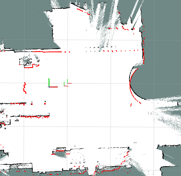
Before optimization

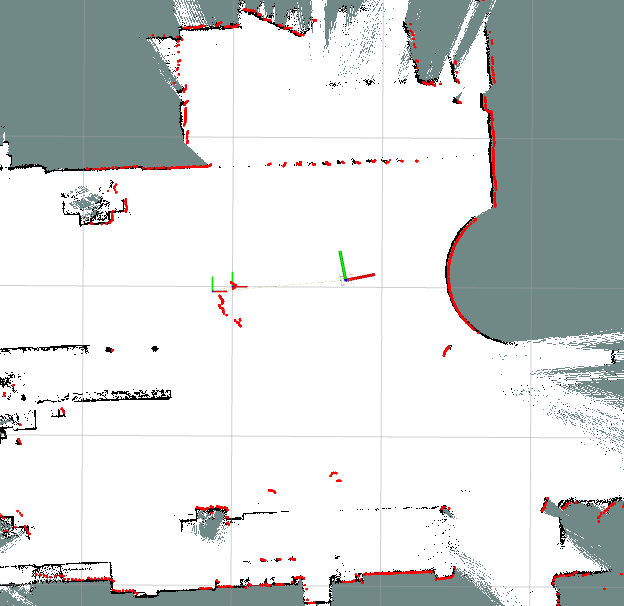
After optimization

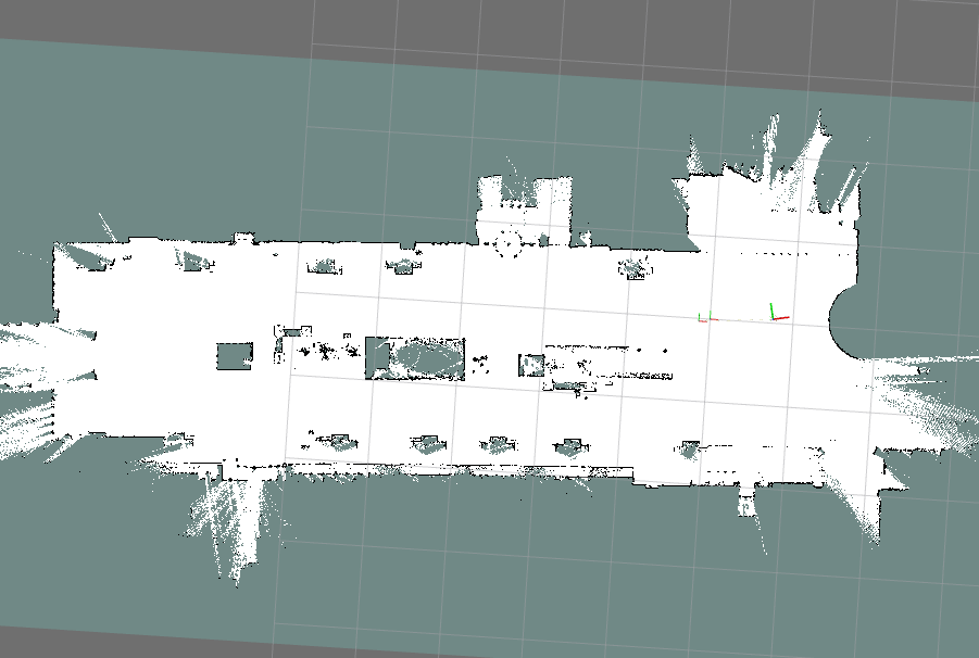
Final map

Final cost

If you look at the final cost, you can see that the cost after the previous optimization is e-15, but the last cost is e-02, which is much larger. The reason is not clear

It is speculated that there is still room for optimization due to the sudden end of the data???

If you know something, you can comment and tell me. Thank you very much

[ INFO] [1637032488.825845405, 1606808848.018522836]: [ceres] Calling ceres for Optimization
Ceres Solver Report: Iterations: 8, Initial cost: 6.562447e-02, Final cost: 5.582333e-15, Termination: CONVERGENCE
[ INFO] [1637032488.850353017, 1606808848.038643242]: [ceres] Optimization finished

[ INFO] [1637032489.159521180, 1606808848.351362847]: [ceres] Calling ceres for Optimization
Ceres Solver Report: Iterations: 8, Initial cost: 2.219165e-02, Final cost: 6.116063e-15, Termination: CONVERGENCE
[ INFO] [1637032489.183078270, 1606808848.371497779]: [ceres] Optimization finished

[ INFO] [1637032489.493828053, 1606808848.683609037]: [ceres] Calling ceres for Optimization
Ceres Solver Report: Iterations: 9, Initial cost: 4.919947e+01, Final cost: 1.920770e-02, Termination: CONVERGENCE
[ INFO] [1637032489.519517167, 1606808848.703747883]: [ceres] Optimization finished

4 Summary

Through this article, we know how to use ceres to build and calculate back-end optimization problems, and experience the map effect and cost value before and after optimization

The next article will use gtsam for back - end optimization calculations