(recently, I was studying the book introduction to algorithms. Before, I liked to write notes by hand, but then I found that I always lost my notes, so I planned to make an electronic version of notes)
(in addition, pseudo code is used in the book, and python code is used in the notes if you need to try.)
2.1 insert sort
Basic idea: regard the sequence to be sorted as two parts (from small to large, for example). The first half is sorted and the second half is disordered. For the first one in disordered order, compare it with the largest number and the second largest number in the first half in turn, and put it in when it is in the right position. Then move the compared number backward by one bit, and the length of the corresponding sorting is increased by one, and those without sorting are reduced by one. For example:
5 | 2 6 4 3 1 ➡️ 2 ? 5: 2 < 5! Insert 2 in front of 5
2 5 | 6 4 3 1 ➡️ 6 ? 5: 6 > 5! Insert 6 behind 5
2 5 6 | 4 3 1 ➡️ 4 ? 6: 4 < 6! four ? 5: 4 < 5! 2 ? 4: 2<4! Insert 4 between 2 and 5
......
In addition, loop invariants are used in the part of proving insertion sorting.
Initialization: before the first iteration of the loop, the proposition is true;
Keep: if it is true before one iteration of the loop, it is still true before the next iteration;
Termination: when the loop terminates, the invariant provides us with a useful property that helps to prove the correctness of the algorithm.
In insertion sorting, the initialization property is reflected in the initial division into two parts. Since the length of the first part is 1, it must also meet the so-called "from small to large" arrangement. The nature of retention is reflected in that if a new number is inserted into the sequence, such as the step of inserting 4, the first sequence is still arranged "from small to large" before and after insertion. The termination property is reflected in the end of the sorting process. The first sequence is arranged "from small to large", which is a "useful property", which can prove that this algorithm is correct.
2.2 analysis algorithm
The efficiency of the algorithm is analyzed and implemented by a hypothetical general single processor computing model random access machine (RAM), which includes arithmetic instructions (addition, subtraction, multiplication, division, rounding), data movement (loading, storage, replication) and control instructions (conditional and unconditional transfer, subroutine call and return), The time of each instruction is constant, which helps us to evaluate the time efficiency of an algorithm.
Because it is an ideal model, the running speed, cache, virtual memory and so on of the computer in the actual calculation will not be considered
By analyzing the complexity of the algorithm, the worst-case running time can be given. Although many times the function of time and data scale is not a simple basic elementary function multiplied by a coefficient, it only needs to consider that it mainly controls the running time when it tends to a large data scale. That is, the higher-order term. Considering its rate of change is often more meaningful than considering its value. In other words, what we are really interested in is the growth rate or magnitude of runtime.
* Why do you often consider the worst case?
- The running state of the algorithm can be effectively characterized (for example, if the result is not seen after the worst case, there may be a bug)
- In many cases, the worst case is the average case. For example, when searching the database, the required data can not be found, but the algorithm is likely to traverse the whole database, that is, the worst case.
2.3 design algorithm
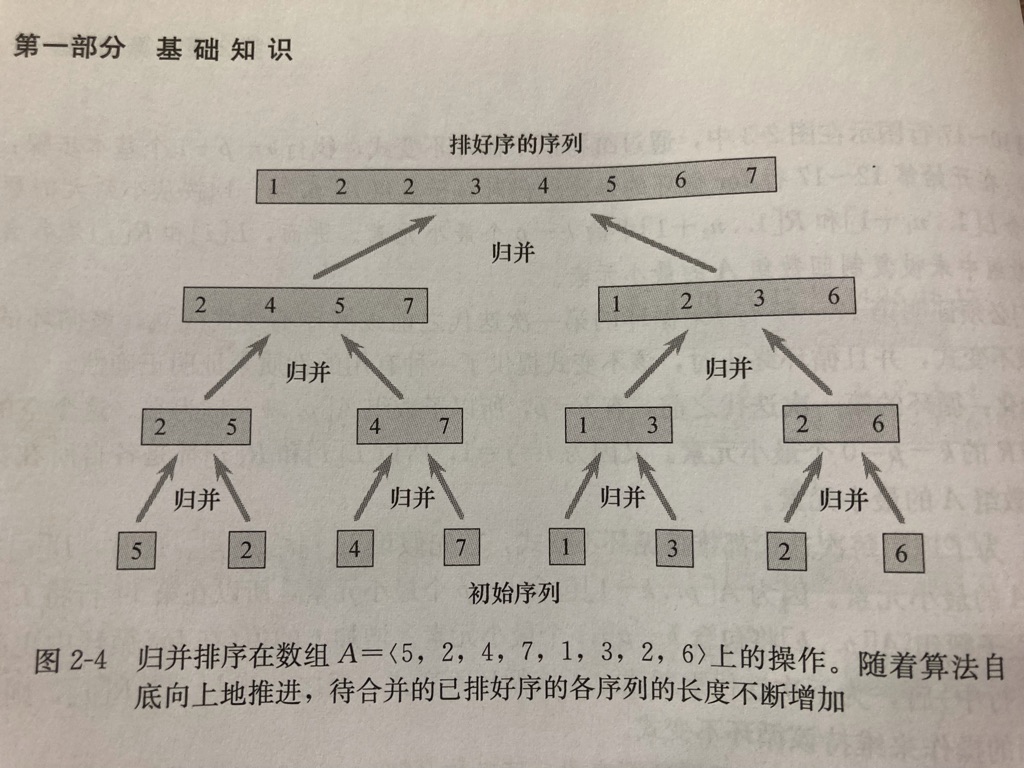
Using the design method of "divide and conquer", we can design a faster method than insertion sorting: merge sorting (recursion)
Basic idea: if there are two ordered list fragments and two position pointers, the final large list fragments are also ordered by comparing the size of the value pointed to by the position pointer and inserting them in turn. And obviously, when the length of these two list fragments is 1, the list is obviously orderly.
Try your own python code:
# Introduction to algorithm 2.3 merge sort exercise code
def guibing(List, p, q, r):
    '''
    Recursive sorting function
    :param List: List waiting to be sorted
    :param p: The lower bound of the list fragment waiting to be sorted
    :param q: The intermediate value of the list fragment waiting to be sorted
    :param r: Upper bound of list fragments waiting to be sorted
    :return: Sorted List
    '''
    if p == q or q == r:
        return List
    ListL = guibing(List, p, (p + q) // 2, q)[p:q]
    ListR = guibing(List, q, (q + r) // 2, r)[q:r]
    print(ListL, ListR)
    ListL.append(1000)
    ListR.append(1000)
    L, R = 0, 0
    list_return = []
    while L < q - p or R < r - q:
        if ListL[L] < ListR[R]:
            list_return.append(ListL[L])
            L += 1
        else:
            list_return.append(ListR[R])
            R += 1
    list_return = List[:p] + list_return + List[r:]
    print(list_return)
    print('-'*80)
    return list_return


guibing([2, 42, 5, 3, 44, 53, 4, 7, 9, 4, 83, 56, 25, 56, 34], 1, 8, 15)
Output:
[5] [3]
[2, 42, 3, 5, 44, 53, 4, 7, 9, 4, 83, 56, 25, 56, 34]
--------------------------------------------------------------------------------
[42] [3, 5]
[2, 3, 5, 42, 44, 53, 4, 7, 9, 4, 83, 56, 25, 56, 34]
--------------------------------------------------------------------------------
[44] [53]
[2, 42, 5, 3, 44, 53, 4, 7, 9, 4, 83, 56, 25, 56, 34]
--------------------------------------------------------------------------------
[4] [7]
[2, 42, 5, 3, 44, 53, 4, 7, 9, 4, 83, 56, 25, 56, 34]
--------------------------------------------------------------------------------
[44, 53] [4, 7]
[2, 42, 5, 3, 4, 7, 44, 53, 9, 4, 83, 56, 25, 56, 34]
--------------------------------------------------------------------------------
[3, 5, 42] [4, 7, 44, 53]
[2, 3, 4, 5, 7, 42, 44, 53, 9, 4, 83, 56, 25, 56, 34]
--------------------------------------------------------------------------------
[4] [83]
[2, 42, 5, 3, 44, 53, 4, 7, 9, 4, 83, 56, 25, 56, 34]
--------------------------------------------------------------------------------
[9] [4, 83]
[2, 42, 5, 3, 44, 53, 4, 7, 4, 9, 83, 56, 25, 56, 34]
--------------------------------------------------------------------------------
[56] [25]
[2, 42, 5, 3, 44, 53, 4, 7, 9, 4, 83, 25, 56, 56, 34]
--------------------------------------------------------------------------------
[56] [34]
[2, 42, 5, 3, 44, 53, 4, 7, 9, 4, 83, 56, 25, 34, 56]
--------------------------------------------------------------------------------
[25, 56] [34, 56]
[2, 42, 5, 3, 44, 53, 4, 7, 9, 4, 83, 25, 34, 56, 56]
--------------------------------------------------------------------------------
[4, 9, 83] [25, 34, 56, 56]
[2, 42, 5, 3, 44, 53, 4, 7, 4, 9, 25, 34, 56, 56, 83]
--------------------------------------------------------------------------------
[3, 4, 5, 7, 42, 44, 53] [4, 9, 25, 34, 56, 56, 83]
[2, 3, 4, 4, 5, 7, 9, 25, 34, 42, 44, 53, 56, 56, 83]
--------------------------------------------------------------------------------

The process has ended with exit code 0
It's easy to see the change in the length of the list and the process of inserting in order.
Steps to solve problems by divide and Conquer:
Decomposition: decompose the original problem into several sub problems
Solution: solve the subproblem. If the scale of the subproblem is small enough, it can be solved directly
Merge: merge subproblems into the solution of the original problem.
Through this recursive method, we can see that a ranking problem will be transformed into two ranking problems with a scale of half the original size, and finally decomposed into many problems with a scale of 1 in exponential form. It is easy to guess that the complexity of the algorithm should be a logarithm related formula. In fact, it is O(nlgn).