This article is shared from Huawei cloud community< [Python artificial intelligence] XVI. Keras environment construction, introduction foundation and case of recurrent neural network >, by eastmount.
1, Why use Keras
Keras is an open source artificial neural network library written by Python. It can be used as a high-level application program interface for Tensorflow, Microsoft cntk and Theano to design, debug, evaluate, apply and visualize the deep learning model. Its main developer is Google engineer Fran ç ois Chollet.
In terms of code structure, keras is written by object-oriented method, which is completely modular and extensible. Its operation mechanism and description documents take user experience and difficulty into account, and try to simplify the implementation difficulty of complex algorithms. Keras supports the mainstream algorithms in the field of modern artificial intelligence, including neural networks with feedforward structure and recursive structure, and can also participate in the construction of statistical learning models through encapsulation. In terms of hardware and development environment, keras supports multi GPU parallel computing under multi operating systems and can be transformed into components under Tensorflow, Microsoft cntk and other systems according to background settings.
As an advanced package of neural network, Keras can quickly build neural network. It has very wide compatibility and is compatible with TensorFlow and Theano.
2, Install Keras and compatible Backend
1. How to install Keras
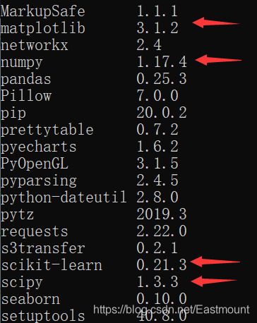
First, you need to ensure that the following two packages are installed:
- Numpy
- Scipy
Call the "pip3 list" command to see that the related packages have been successfully installed.
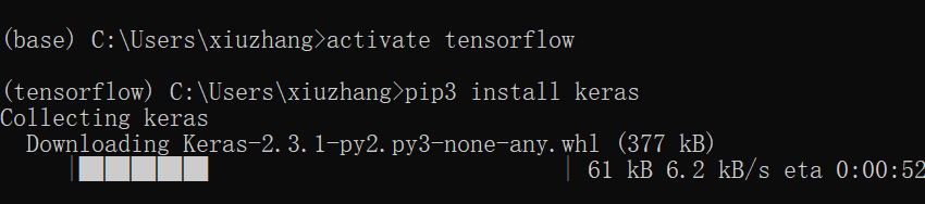
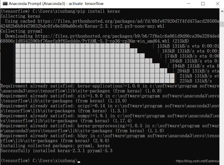
Then install through "pip3 install keras". The author uses Python 3.6 under Anaconda.
activate tensorflow
pip3 install keras
pip install keras
See this article for the construction process:
The installation is shown in the figure below:
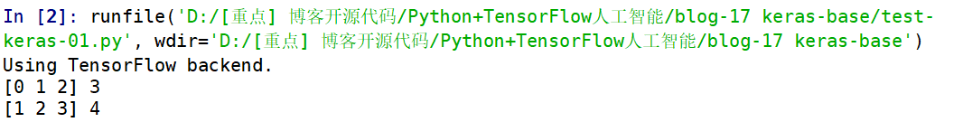
After the installation is successful, we try a simple code. Open Anaconda, select the built "tensorflow" environment, and run Spyder.

The test code is as follows:
# -*- coding: utf-8 -*-
"""
Created on Fri Feb 14 16:43:21 2020
@author: Eastmount CSDN
"""
import numpy as np
from keras.preprocessing.sequence import TimeseriesGenerator

# time series
y = np.array(range(5))
tg = TimeseriesGenerator(y, y, length=3, sampling_rate=1)
for i in zip(*tg[0]):
    print(*i)
The running results are shown in the figure below. What does "Using TensorFlow backend." mean?
2. Compatible with Backend
Backend means that Keras performs operations based on a framework, including TensorFlow or Theano. The above code uses TensorFlow to perform operations. The neural network to be explained later is also built based on TensorFlow or Theano.
How do I view the Backend? When we import the Keras extension package, it will have corresponding prompts. For example, Theano is used in the following figure to build the underlying neural network.

What if you want to change to TensorFlow?
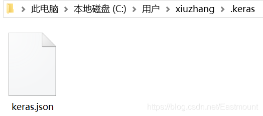
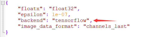
- First, find the file "keras/keras.json" and open it. All the backend information is stored here. Each time the Keras package is imported, the backend of the "keras.json" file will be detected. Then we try to modify it.
- The second method is to enter the following command on the command line. Each time you run the script, it will directly help you modify it into a temporary TensorFlow.
import os
os.environ['KERAS_BACKEND']='tensorflow'
import keras
3, Vernacular neural network
It is still necessary to popularize this part again. Refer to the introduction of neural network in "don't bother God" Netease cloud course, which is clear and thorough. It is recommended that you read it. Let's go! Let's enter the world of neural network and TensorFlow.
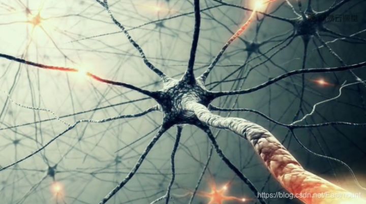
First, what is Neural Networks?
Computer neural network is a kind of mathematical model or computer model that imitates the structure and function of biological neural network or animal neural center, especially the brain. Neural network is connected and calculated by a large number of neurons. In most cases, artificial neural network can change the internal structure on the basis of external information, which is an adaptive process.
Modern neural network is a tool based on traditional statistical modeling. It is often used to model the complex relationship between input and output, or explore the mode between data. Neural network is an operation model, which is composed of a large number of nodes or neurons and their connections. Like human neurons, they are responsible for transmitting and processing information. Neurons can also be trained or strengthened to form a fixed nerve form and respond more strongly to special information.
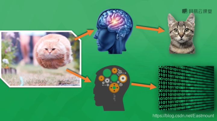
How do neural networks work?
As shown in the above figure, whether it is a jumping cat or a quiet thinking cat, you know it is a cat, because your brain has been told that the cat with round eyes, furry and sharp ears is a cat. You judge it as a cat through the mature visual nervous system. Computers are the same. Through continuous training, they tell which are cats, dogs and pigs. They will summarize these learning judgments through mathematical models and finally classify them in the form of Mathematics (0 or 1). At present, Google and Baidu image search can clearly identify things, which is due to the rapid development of computer nervous system.
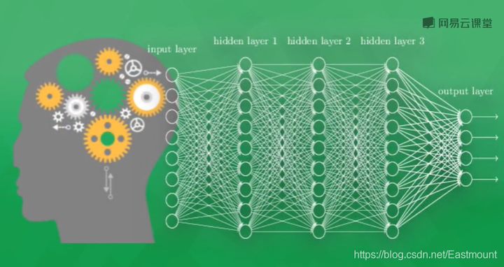
The neural network system consists of multiple neural layers. In order to distinguish different neural layers, we are divided into:
- Input layer: the neural layer that directly receives information, such as a picture of a cat
- Output layer: information is transferred and analyzed in neurons to form output results. Through the output results of this layer, we can see the computer's cognition of things
- Hidden layer: each layer composed of many neuron connections between the input and output layers can have multiple layers, which is responsible for the processing of incoming information. After multi-layer processing, the understanding of cognition can be derived
Examples of neural networks
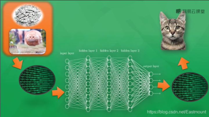
As shown in the figure below, generally speaking, the things processed by computers are different from human beings. Whether it is sound, picture or text, they can only appear in the computer neural network as the number 0 or 1. The pictures seen by the neural network are actually a pile of numbers. The processing of numbers finally generates another pile of numbers, which has certain cognitive significance. Through a little processing, we can know whether the computer judges whether the picture is a cat or a dog.
How do computers train?
First, we need a lot of data. For example, if we need a computer to judge whether it is a cat or a dog, we need to prepare tens of millions of labeled pictures, and then conduct tens of millions of training. The computer judges the cat through training or reinforcement learning, and converts the acquired features into mathematical form.

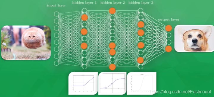
What we need to do is just show the computer the picture, and then let it give us an immature and inaccurate answer. It is possible that 10% of the answers in 100 times are correct. If the picture shown to the computer is a running cat (as shown in the figure below), the computer may recognize it as a dog. Although it recognizes the error, this error is very valuable to the computer. You can use this wrong experience as a good teacher and continue to learn the experience.

So how do computers learn from experience?
It compares the difference between the predicted answer and the real answer, and then transfers the difference back, modifies the weight of neurons, and makes each neuron change a little in the right direction. In this way, by the next recognition, the accuracy of computer recognition will be improved through all improved neural networks. In the end, every little bit and tens of millions of training will take a big step in the right direction.

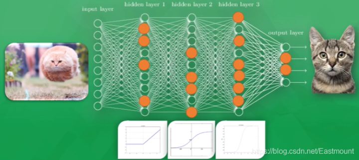
Finally, when it comes to the acceptance results, when the computer displays the picture of the cat again, it can correctly predict that it is a cat.

What is the excitation function?
Then take a further look at how neural networks are trained. It turns out that every neuron in the computer has its own Active Function. We can use these incentive functions to give the computer a stimulating behavior. When we first showed the computer a running cat, only some neurons in the neural network were activated or excited. The information transmitted by activation is the information that the computer attaches most importance to and the most valuable information for the output results.
If the prediction result is a dog, the parameters of all neurons will be adjusted. At this time, some neurons that are easy to be activated will become dull, while others will become sensitive, which shows that all neuron parameters are being modified and become sensitive to the really important information of the picture, so that the changed parameters can gradually predict the correct answer, It is a cat. This is the processing process of neural network.
4, Keras builds regression neural network
Recommended earlier: [Python artificial intelligence] II. TensorFlow foundation and univariate linear prediction case , the final output result is shown in the figure below:
1. Import expansion pack
Sequential (sequential model) means to establish the model in order. It is the simplest linear and structural order from beginning to end. It is not forked. It is a linear stack of multiple network layers. Density is an attribute in layers, which represents a fully connected layer. Keras can also implement various layers, including core layer, revolution volume layer, Pooling layer and other very rich and interesting network structures.
import numpy as np
from keras.models import Sequential
from keras.layers import Dense
import matplotlib.pyplot as plt
2. Create scatter chart data
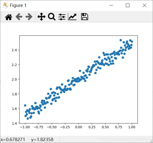
Generate 200 scatter points randomly through numpy.linspace, build virtual data with y=0.5*x+2, and call np.random.normal(0, 0.05, (200,)) to increase noise.
import numpy as np
from keras.models import Sequential
from keras.layers import Dense
import matplotlib.pyplot as plt

#---------------------------Create scatter data---------------------------
# input
X = np.linspace(-1, 1, 200)
# Randomized data
np.random.shuffle(X)
# output
y = 0.5*X + 2 + np.random.normal(0, 0.05, (200,)) #Noise mean value 0, variance 0.05
# Scatter plot
plt.scatter(X, y)
plt.show()

# Data set division (training set test set)
X_train, y_train = X[:160], y[:160]  # First 160 scatter points
X_test, y_test = X[160:], y[160:]    # Last 40 scatter points
Here, the scatter diagram is simply drawn through matplotlib, and the output result is shown in the figure below, which basically meets the following requirements: y = 0.5*x + 2 + noise.
3. Add neural network layer
- Create a Sequential model.
- Add a neural network layer. In Keras, the operation of adding layers is very simple. You can call the model. Add (density (output_dim = 1, input_dim = 1)) function to add layers. Note that if another neural layer is added, the output of the previous layer is the input data of the next layer by default. At this time, it is not necessary to define the input_ Dim, such as model.add(Dense(output_dim=1,)).
- Build the model and select loss function and optimization method.
#----------------------------Add nerve layer------------------------------
# Create model
model = Sequential()

# Increase the number of outputs and inputs of the full connection layer (both 1)
model.add(Dense(output_dim=1, input_dim=1))

# Build a model and select loss function and optimization method
# mse represents quadratic error and sgd represents out of order gradient descent optimizer
model.compile(loss='mse', optimizer='sgd')
PS: do you think the Keras code is much simpler than TensorFlow and Theano, but I suggest you learn the former first and then go deep into Keras.
4. Train and output error
print("train")
# Learn 300 times
for step in range(301):
    # The return value of batch training data is error
    cost = model.train_on_batch(X_train, y_train)
    # Output error every 100 steps
    if step % 100 == 0:
        print('train cost:', cost)
5. Test the neural network and output error \ weight and bias
print("test")
# Run the model test and pass in 40 test scatter points at a time
cost = model.evaluate(X_test, y_test, batch_size=40)
# output error
print("test cost:", cost)
# Get weights and errors layers[0] represents the first neural layer (i.e. Dense)
W, b = model.layers[0].get_weights()
# Output weights and offsets
print("weights:", W)
print("biases:", b)
6. Draw prediction graph
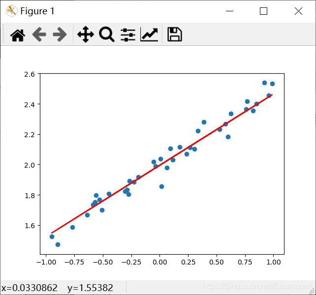
y_pred = model.predict(X_test)
plt.scatter(X_test, y_test)
plt.plot(X_test, y_pred)
plt.show()
The output results are as follows:
The error decreased from 4.002261 to 0.0030148015, indicating that knowledge has been learned. At the same time, the error is 0.47052705, which is close to our initial value of 0.5, and the offset is 1.9944116, which is also close to 2.
train
train cost: 4.002261
train cost: 0.07719966
train cost: 0.005076804
train cost: 0.0030148015
test
40/40 [==============================] - 0s 1ms/step
test cost: 0.0028453178238123655
weights: [[0.47052705]]
biases: [1.9944116]
The complete code is as follows:
# -*- coding: utf-8 -*-
"""
Created on Fri Feb 14 16:43:21 2020
@author: Eastmount CSDN YXZ
O(∩_∩)O Wuhan Fighting!!!
"""
import numpy as np
from keras.models import Sequential
from keras.layers import Dense
import matplotlib.pyplot as plt
#---------------------------Create scatter data---------------------------
# input
X = np.linspace(-1, 1, 200)
# Randomized data
np.random.shuffle(X)
# output
y = 0.5*X + 2 + np.random.normal(0, 0.05, (200,)) #Noise mean value 0, variance 0.05
# Scatter plot
# plt.scatter(X, y)
# plt.show()
# Data set division (training set test set)
X_train, y_train = X[:160], y[:160] # First 160 scatter points
X_test, y_test = X[160:], y[160:] # Last 40 scatter points
#----------------------------Add nerve layer------------------------------
# Create model
model = Sequential()
# Increase the number of outputs and inputs of the full connection layer (both 1)
model.add(Dense(output_dim=1, input_dim=1))
# Build a model and select loss function and optimization method
# mse represents quadratic error and sgd represents out of order gradient descent optimizer
model.compile(loss='mse', optimizer='sgd')
#--------------------------------Traning----------------------------
print("train")
# Learn 300 times
for step in range(301):
# The return value of batch training data is error
cost = model.train_on_batch(X_train, y_train)
# Output error every 100 steps
if step % 100 == 0:
print('train cost:', cost)
#--------------------------------Test-------------------------------
print("test")
# Run the model test and pass in 40 test scatter points at a time
cost = model.evaluate(X_test, y_test, batch_size=40)
# output error
print("test cost:", cost)
# Get weights and errors layers[0] represents the first neural layer (i.e. Dense)
W, b = model.layers[0].get_weights()
# Output weights and offsets
print("weights:", W)
print("biases:", b)
#------------------------------Draw prediction graph-----------------------------
y_pred = model.predict(X_test)
plt.scatter(X_test, y_test)
plt.plot(X_test, y_pred, "red")
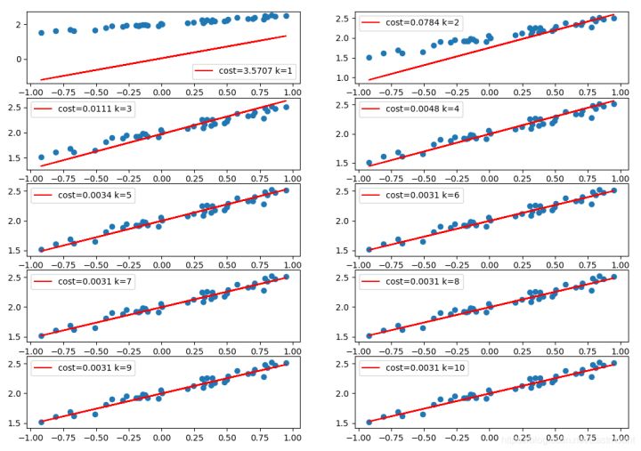
plt.show()The following supplementary code compares the fitted lines in each training stage. It can be seen that with the increase of training times, the error decreases gradually, and the fitted lines are getting better and better.
# -*- coding: utf-8 -*-
"""
Created on Fri Feb 14 16:43:21 2020
@author: Eastmount CSDN YXZ
"""
import numpy as np
from keras.models import Sequential
from keras.layers import Dense
import matplotlib.pyplot as plt

#---------------------------Create scatter data---------------------------
# input
X = np.linspace(-1, 1, 200)
# Randomized data
np.random.shuffle(X)
# output
y = 0.5*X + 2 + np.random.normal(0, 0.05, (200,)) #Noise mean value 0, variance 0.05
# Scatter plot
# plt.scatter(X, y)
# plt.show()

# Data set division (training set test set)
X_train, y_train = X[:160], y[:160]  # First 160 scatter points
X_test, y_test = X[160:], y[160:]    # Last 40 scatter points

#----------------------------Add nerve layer------------------------------
# Create model
model = Sequential()

# Increase the number of outputs and inputs of the full connection layer (both 1)
model.add(Dense(output_dim=1, input_dim=1))

# Build a model and select loss function and optimization method
# mse represents quadratic error and sgd represents out of order gradient descent optimizer
model.compile(loss='mse', optimizer='sgd')

#--------------------------------Traning----------------------------
print("train")
k = 0
# Learn 1000 times
for step in range(1000):
    # The return value of batch training data is error
    cost = model.train_on_batch(X_train, y_train)
    # Output error every 100 steps
    if step % 100 == 0:
        print('train cost:', cost)

        #-----------------------------------------------------------
        # Run the model test and pass in 40 test scatter points at a time
        cost = model.evaluate(X_test, y_test, batch_size=40)
        # output error
        print("test cost:", cost)
        # Get weights and errors layers[0] represents the first neural layer (i.e. Dense)
        W, b = model.layers[0].get_weights()
        # Output weights and offsets
        print("weights:", W)
        print("biases:", b)

        #-----------------------------------------------------------
        # Visual drawing
        k = k + 1
        plt.subplot(5, 2, k)
        y_pred = model.predict(X_test)
        plt.scatter(X_test, y_test)
        plt.plot(X_test, y_pred, "red", label='cost=%.4f k=%d' %(cost,k))
        plt.legend()

plt.show()
Click focus to learn about Huawei cloud's new technologies for the first time~