[note]: the data of two books are loaded here, both of which are mentioned in Li Mu's divine book. Since the code encapsulated by Mu Shen is loaded Time machine, I copied the code of the previous two blogs here to load the Star Wars dataset. The following content is a reproduction of Mu God's curriculum and code. I will mark the knowledge points in yellow.

%matplotlib inline
import math
import torch
from torch import nn
from torch.nn import functional as F
from d2l import torch as d2l 
import re
import collections
import random

1. Data loading and conversion

1.1 load the book Time machine

# Load data
batch_size,num_steps = 32,35
train_iter,vocab = d2l.load_data_time_machine(batch_size,num_steps)

# Encode the number of each mark
# The unique codes with indexes 0 and 2 are as follows
F.one_hot(torch.tensor([0,2]),len(vocab))

tensor([[1, 0, 0, 0, 0, 0, 0, 0, 0, 0, 0, 0, 0, 0, 0, 0, 0, 0, 0, 0, 0, 0, 0, 0,
         0, 0, 0, 0],
        [0, 0, 1, 0, 0, 0, 0, 0, 0, 0, 0, 0, 0, 0, 0, 0, 0, 0, 0, 0, 0, 0, 0, 0,
         0, 0, 0, 0]])

  the small batch shape we sample each time is (batch size, time steps). one_hot coding converts such a small batch into a three-dimensional tensor, and the last dimension is equal to the vocabulary size (len(vocab)). We often replace the input dimensions to obtain the output of shapes (time steps, batch size, vocabulary size). This will make it easier for us to update the hidden state of small batches step by step through the outermost dimension. (imagine the data on each time step we input during training later. The transposed data is convenient for us to read in python and has a certain calculation acceleration effect)

X = torch.arange(10).reshape((2, 5))
F.one_hot(X.T, 28).shape

torch.Size([5, 2, 28])

1.2 reading the Star Wars Book dataset

Manually modify the previous code a little. There is no encapsulation for easy viewing

def read_book(dir):
    """The preprocessing operation here is violent. Punctuation and special characters are eliminated, leaving only 26 letters and spaces"""
    with open(dir,'r') as f:
        lines = f.readlines()
    return [re.sub('[^A-Za-z]+',' ',line).strip().lower() for line in lines]

def tokenize(lines,token='word'):
    if token=="word":
        return [line.split() for line in lines]
    elif token =="char":
        return [list(line) for line in lines]
    else:
        print("Error:Unknown token type:"+token)

        lines = read_book('./data/RNN/36-0.txt') 
        
def count_corpus(tokens):
    """Frequency of statistical markers: here tokens Yes 1 D List or 2 D list"""
    if len(tokens) ==0 or isinstance(tokens[0],list):
        # Flatten tokens into a list filled with tags
        tokens = [token for line in tokens for token in line]
    return collections.Counter(tokens)

class Vocab:
    """Building a text Thesaurus"""
    def __init__(self,tokens=None,min_freq=0,reserved_tokens=None):
        if tokens is None:
            tokens=[]
        if reserved_tokens is None:
            reserved_tokens = []
        # Sort by frequency
        counter = count_corpus(tokens)
        self.token_freqs = sorted(counter.items(),key=lambda x:x[1],reverse=True)
        
        # Index of unknown tag is 0
        self.unk , uniq_tokens = 0, ['<unk>']+reserved_tokens
        uniq_tokens += [token for token,freq in self.token_freqs
                       if freq >= min_freq and token not in uniq_tokens]
        self.idx_to_token,self.token_to_idx = [],dict() # Find tag by index and find index by tag
        for token in uniq_tokens:
            self.idx_to_token.append(token)
            self.token_to_idx[token] = len(self.idx_to_token)-1
            
    def __len__(self):
        return len(self.idx_to_token)
    
    def __getitem__(self,tokens):
        """Convert to one by one item Output"""
        if not isinstance(tokens,(list,tuple)):
            return self.token_to_idx.get(tokens,self.unk)
        return [self.__getitem__(token) for token in tokens]
    
    def to_tokens(self,indices):
        """If single index Direct output, if yes list perhaps tuple Iterative output"""
        if not isinstance(indices,(list,tuple)):
            return self.idx_to_token[indices]
        return [self.idx_to_token[index] for index in indices]
    
def load_corpus_book(max_tokens=-1):
    """return book Tag index list and glossary in dataset"""
    lines = read_book('./data/RNN/36-0.txt')
    tokens = tokenize(lines,'char')
    vocab = Vocab(tokens)
    # Because every text line in the dataset is not necessarily a sentence or paragraph
    # So flatten all text lines into a list
    corpus = [vocab[token] for line in tokens for token in line]
    if max_tokens >0:
        corpus = corpus[:max_tokens]
    return corpus,vocab

def seq_data_iter_random(corpus,batch_size,num_steps):
    """Random sampling is used to generate a small batch of quantum sequences"""
    # The sequence is partitioned from the random offset. The random range includes ` num_steps - 1`
    corpus = corpus[random.randint(0, num_steps - 1):]
    # Minus 1 is because we need to consider labels
    num_subseqs = (len(corpus) - 1) // num_steps
    # Length ` num_ Start index of the subsequence of steps'
    initial_indices = list(range(0, num_subseqs * num_steps, num_steps))
    # In the iterative process of random sampling,
    # Subsequences from two adjacent, random, small batches are not necessarily adjacent to the original sequence
    random.shuffle(initial_indices)

    def data(pos):
        # The length returned from the 'pos' position is ` num_ Sequence of steps
        return corpus[pos:pos + num_steps]

    num_batches = num_subseqs // batch_size
    for i in range(0, batch_size * num_batches, batch_size):
        # Here, ` initial_ Indexes ` random start indexes containing subsequences
        initial_indices_per_batch = initial_indices[i:i + batch_size]
        X = [data(j) for j in initial_indices_per_batch]
        Y = [data(j + 1) for j in initial_indices_per_batch]
        yield torch.tensor(X), torch.tensor(Y)
        
def seq_data_iter_sequential(corpus,batch_size,num_steps):
    """Using sequential partitioning to generate a small batch of quantum sequences"""
    # Divide the sequence from a random offset
    offset = random.randint(0,num_steps)
    num_tokens = ((len(corpus)- offset -1)//batch_size)*batch_size
    Xs = torch.tensor(corpus[offset:offset+num_tokens])
    Ys = torch.tensor(corpus[offset+1:offset+num_tokens+1])
    Xs,Ys = Xs.reshape(batch_size,-1),Ys.reshape(batch_size,-1)
    num_batches = Xs.shape[1]//num_steps
    for i in range(0,num_steps*num_batches,num_steps):
        X = Xs[:,i:i+num_steps]
        Y = Ys[:,i:i+num_steps]
        yield X,Y

class SeqDataLoader:  #@save
    """An iterator that loads sequence data."""
    def __init__(self, batch_size, num_steps, use_random_iter, max_tokens):
        if use_random_iter:
            self.data_iter_fn = seq_data_iter_random
        else:
            self.data_iter_fn = seq_data_iter_sequential
        self.corpus, self.vocab = load_corpus_book(max_tokens)
        self.batch_size, self.num_steps = batch_size, num_steps

    def __iter__(self):
        return self.data_iter_fn(self.corpus, self.batch_size, self.num_steps)
        
# Define function load_data_book returns both a data iterator and a vocabulary
def load_data_book(batch_size, num_steps,  #@save
                           use_random_iter=False, max_tokens=10000):
    """Returns the iterator and vocabulary of the time machine dataset."""
    data_iter = SeqDataLoader(batch_size, num_steps, use_random_iter,max_tokens)
    return data_iter, data_iter.vocab

# Load data
batch_size,num_steps = 32,35
train_iter,vocab = load_data_book(batch_size,num_steps)

2. Initialize model parameters

num_hiddens is an adjustable super parameter. When training the network model, the input and output come from the same thesaurus, so it has the same dimension, which is equal to the size of the thesaurus

def get_params(vocab_size,num_hiddens,device):
    num_inputs = num_outputs = vocab_size
    
    def normal(shape):
        return torch.randn(size=shape,device=device)*0.01
    
    # Hidden layer parameters
    W_xh = normal((num_inputs,num_hiddens)) # Map input to hidden layers
    W_hh = normal((num_hiddens,num_hiddens)) # Hidden variables from the previous time to the next time
    b_h = torch.zeros(num_hiddens,device=device) # bias for each hidden variable
    
    # Output layer
    W_hq = normal((num_hiddens,num_outputs)) # Hide variables to output
    b_q = torch.zeros(num_outputs,device=device)
    
    # Additional gradient
    params = [W_xh,W_hh,b_h,W_hq,b_q]
    for param in params:
        param.requires_grad_(True)
    return params

3. Cyclic neural network model

  in order to define the recurrent neural network model, we first need a function to return the hidden state during initialization. It returns a tensor, all filled with 0, and its shape is (batch size, number of hidden units). Using tuples makes it easier to handle situations where the hidden state contains multiple variables.

def init_rnn_state(batch_size,num_hiddens,device):
    return (torch.zeros((batch_size,num_hiddens),device=device),)

  use the rnn function to define how to calculate the hidden state and output in a time step. Note that the recurrent neural network model circulates through the outermost dimension inputs, so as to update the small batch of hidden state H step by step. The activation function uses the tanh function. As described in the multi-layer perceptron chapter, when the elements are evenly distributed in real numbers, the average value of tanh is 0

def rnn(inputs, state, params):
    # `Shape of inputs: (` number of time steps', 'batch size', 'thesaurus size')
    W_xh, W_hh, b_h, W_hq, b_q = params
    H, = state # H is the hidden state of the previous time
    outputs = []
    # `Shape of X: (` batch size ', ` thesaurus size')
    for X in inputs:
        """Traverse the data in chronological order"""
        H = torch.tanh(torch.mm(X, W_xh) + torch.mm(H, W_hh) + b_h)
        Y = torch.mm(H, W_hq) + b_q
        outputs.append(Y)
    return torch.cat(outputs, dim=0), (H,)

# Use a class to integrate all the above functions and store the model parameters of RNN
class RNNModelScratch:  #@save
    """Cyclic neural network model implemented from scratch"""
    def __init__(self, vocab_size, num_hiddens, device, get_params,
                 init_state, forward_fn):
        self.vocab_size, self.num_hiddens = vocab_size, num_hiddens
        self.params = get_params(vocab_size, num_hiddens, device)
        self.init_state, self.forward_fn = init_state, forward_fn

    def __call__(self, X, state):
        X = F.one_hot(X.T, self.vocab_size).type(torch.float32)
        return self.forward_fn(X, state, self.params)

    def begin_state(self, batch_size, device):
        return self.init_state(batch_size, self.num_hiddens, device)

#Check whether the shape of the output is correct to ensure that the dimension of the hidden state remains unchanged
num_hiddens = 512
net = RNNModelScratch(len(vocab),num_hiddens,d2l.try_gpu(),get_params,init_rnn_state,rnn)
state = net.begin_state(X.shape[0],d2l.try_gpu())
Y,new_state = net(X.to(d2l.try_gpu()),state)
Y.shape, len(new_state), new_state[0].shape

(torch.Size([10, 28]), 1, torch.Size([2, 512]))

The output shape is (time steps * batch size, vocabulary size), while the shape of the hidden state remains unchanged, that is (batch size, number of hidden units)

4. Forecast

    define the prediction function to generate new characters after the prefix provided by the user. Prefix is a string containing multiple characters. When looping through these starting characters in prefix, the hidden state is continuously passed to the next time step without generating any output.

   this is called a "warm-up period", during which the model updates itself (for example, updates the hidden state), but does not predict.
After the forecast period, the hidden state is better than the initial value at the beginning.

def predict(prefix,num_preds,net,vocab,device):
    """stay prefix Generate new characters after"""
    state = net.begin_state(batch_size=1,device=device)
    outputs = [vocab[prefix[0]]]
    get_input = lambda: torch.tensor([outputs[-1]], device=device).reshape((1, 1))
    
    for y in prefix[1:]: #Preheating period
        _,state = net(get_input(),state)
        outputs.append(vocab[y])
    
    for _ in range(num_preds): # Progress ` num_preds ` step prediction
        y,state = net(get_input(),state)
        outputs.append(int(y.argmax(dim=1).reshape(1)))
    return "".join([vocab.idx_to_token[i] for i in outputs])

predict('time traveller ', 10, net, vocab, d2l.try_gpu())

'time traveller awmjvgtmjv'

5. Gradient cutting

  for length T T For the sequence of T, we calculate these in the iteration T T The gradient on T time steps, resulting in a length of O ( T ) \mathcal{O}(T) Matrix multiplication chain of O(T). When T T When T is large, it may lead to numerical instability, such as gradient explosion or gradient disappearance. Therefore, the recurrent neural network model often needs additional help to stabilize the training.

   generally speaking, when solving optimization problems, we take update steps for model parameters, such as in vector form x \mathbf{x} x, negative gradient in small batch g \mathbf{g} g direction. For example, use η > 0 \eta > 0 η> 0 as the learning rate, in one iteration, we will x \mathbf{x} x updated to x − η g \mathbf{x} - \eta \mathbf{g} x− η g. Let's further assume the objective function f f f performs well, for example, the Lipschitz continuous constant L L L. That is, for any x \mathbf{x} x and y \mathbf{y} y we have:

∣ f ( x ) − f ( y ) ∣ ≤ L ∥ x − y ∥ . |f(\mathbf{x}) - f(\mathbf{y})| \leq L \|\mathbf{x} - \mathbf{y}\|. ∣f(x)−f(y)∣≤L∥x−y∥.

   in this case, we can reasonably assume that if we pass the parameter vector η g \eta \mathbf{g} η g update, then:

∣ f ( x ) − f ( x − η g ) ∣ ≤ L η ∥ g ∥ , |f(\mathbf{x}) - f(\mathbf{x} - \eta\mathbf{g})| \leq L \eta\|\mathbf{g}\|, ∣f(x)−f(x−ηg)∣≤Lη∥g∥,

  this means that we will not observe more than L η ∥ g ∥ L \eta \|\mathbf{g}\| L η Change of ‖ g ‖. This is both a curse and a blessing. On the curse side, it limits the speed of progress; On the blessing side, it limits the extent to which things will go wrong if we move in the wrong direction.

  sometimes the gradient may be large, and the optimization algorithm may not converge. We can reduce η \eta η Learning rate to solve this problem. But what if we rarely get large gradients? In this case, this approach seems totally unfounded. A popular alternative is by incorporating gradients g \mathbf{g} G projects back to a ball of a given radius (e.g θ \theta θ) To crop the gradient g \mathbf{g} g. The following formula:

g ← min ⁡ ( 1 , θ ∥ g ∥ ) g . \mathbf{g} \leftarrow \min\left(1, \frac{\theta}{\|\mathbf{g}\|}\right) \mathbf{g}. g←min(1,∥g∥θ​)g.

  by doing so, we know that the gradient norm will never exceed θ \theta θ， And the updated gradient is completely consistent with g \mathbf{g} It also has an ideal side effect of limiting any given small batch (and any given sample in it) This gives the model a certain degree of robustness. Gradient clipping provides a fast method to repair gradient explosion. Although it can not completely solve the problem, it is one of many technologies to alleviate the problem.

   next, we define a function to cut the gradient of models implemented from scratch or built by high-level API s. Also note that we calculate the gradient norm of all model parameters.

def grad_clipping(net, theta):  #@save
    """Crop gradient."""
    if isinstance(net, nn.Module):
        params = [p for p in net.parameters() if p.requires_grad]
    else:
        params = net.params
    norm = torch.sqrt(sum(torch.sum((p.grad**2)) for p in params))
    if norm > theta:
        for param in params:
            param.grad[:] *= theta / norm

6. Training

  before training the model, let's define a function to train the model with only one iteration cycle. It is different from the way we train the softmax regression model in three ways:

1. Different sampling methods (random sampling and sequential partitioning) of sequential data will lead to the difference of hidden state initialization.
2. We crop the gradient before updating the model parameters, which ensures that the model will not diverge even if the gradient explodes at a certain point in the training process.
3. We use confusion degree to evaluate the model, which ensures the comparability of sequences with different lengths.

   specifically, when using sequential partitioning, we only initialize the hidden state at the beginning of each iteration cycle. Due to the i t h i^\mathrm{th} ith subsequence samples and current i t h i^\mathrm{th} The ith subsequence samples are adjacent, so the hidden state at the end of the current small batch will be used to initialize the hidden state at the beginning of the next small batch. In this way, the sequence history information stored in the hidden state can flow through the adjacent subsequences in an iteration cycle. However, any point of hidden state calculation depends on all the previous small batches in the same iteration cycle, which makes In order to reduce the amount of calculation, we separate the gradient before dealing with any small batch, so that the gradient calculation in the hidden state is always limited to a small batch of time steps.

  when using random sampling, we need to reinitialize the hidden state for each iteration cycle, because each sample is sampled at a random position.

def train_epoch(net, train_iter, loss, updater, device, use_random_iter):
    """The training model has an iterative cycle."""
    state, timer = None, d2l.Timer()
    metric = d2l.Accumulator(2)  # Sum of training losses, number of marks
    for X, Y in train_iter:
        if state is None or use_random_iter:
            # Initialize at first iteration or when using random sampling ` state`
            state = net.begin_state(batch_size=X.shape[0], device=device)
        else:
            if isinstance(net, nn.Module) and not isinstance(state, tuple):
                # `state ` is a tensor for ` nn.GRU '
                state.detach_()
            else:
                # `state ` is a tensor for ` nn.LSTM 'or for our model implemented from scratch
                for s in state:
                    s.detach_()
        y = Y.T.reshape(-1)
        X, y = X.to(device), y.to(device)
        y_hat, state = net(X, state)
        l = loss(y_hat, y.long()).mean()
        if isinstance(updater, torch.optim.Optimizer):
            updater.zero_grad()
            l.backward()
            grad_clipping(net, 1)
            updater.step()
        else:
            l.backward()
            grad_clipping(net, 1)
            # Because the 'mean' function has been called
            updater(batch_size=1)
        metric.add(l * y.numel(), y.numel())
    return math.exp(metric[0] / metric[1]), metric[1] / timer.stop()

#@save
def train(net, train_iter, vocab, lr, num_epochs, device,use_random_iter=False):
    """Training model"""
    loss = nn.CrossEntropyLoss()
    animator = d2l.Animator(xlabel='epoch', ylabel='perplexity',
                            legend=['train'], xlim=[10, num_epochs])
    # initialization
    if isinstance(net, nn.Module):
        updater = torch.optim.SGD(net.parameters(), lr)
    else:
        updater = lambda batch_size: d2l.sgd(net.params, lr, batch_size)
    predict_train = lambda prefix: predict(prefix, 50, net, vocab, device)
    # Training and forecasting
    for epoch in range(num_epochs):
        ppl, speed = train_epoch(net, train_iter, loss, updater, device,
                                     use_random_iter)
        if (epoch + 1) % 10 == 0:
            print(predict_train('time traveller'))
            animator.add(epoch + 1, [ppl])
    print(f'Confusion degree {ppl:.1f}, {speed:.1f} sign/second {str(device)}')
    print(predict_train('the planet mars i scarcely'))
    print(predict_train('scarcely'))

Now we can train the recurrent neural network model. Because we only use 10000 markers in the data set, the model needs more iteration cycles to converge better.

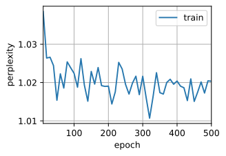
num_epochs, lr = 500, 1
train(net, train_iter, vocab, lr, num_epochs, d2l.try_gpu())

Confusion 1.0, 172140.2 sign/second cuda:0
the planet mars i scarcely need remind the reader revolves about thesun at a
scarcely ore seventh ofthe volume of the earth must have a

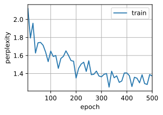
Finally, let's examine the results using the random sampling method.

train(net, train_iter, vocab, lr, num_epochs, d2l.try_gpu(),use_random_iter=True)

Confusion 1.4, 172089.0 sign/second cuda:0
<unk>he planet <unk>ars<unk> <unk> scarcely one seventh ofthe volume of the earth must have a
scarcely one seventh ofthe volume of the earth must have a

Summary

• We can train a character level language model based on cyclic neural network to generate text according to the text prefix provided by the user.
• A simple recurrent neural network language model includes input coding, recurrent neural network model and output generation.
• Cyclic neural network model needs state initialization to train, although random sampling and sequential division use different methods.
• When using sequential partitioning, we need to separate gradients to reduce the amount of computation.
• The warm-up period allows the model to update itself before making any predictions (for example, to obtain a better hidden state than the initial value).
• Gradient clipping can prevent gradient explosion, but it can't deal with gradient disappearance.

practice

1. It shows that single hot coding is equivalent to selecting different embedding for each object.
2. The confusion is improved by adjusting the super parameters (such as the number of iteration cycles, the number of hidden units, the number of time steps in small batches, the learning rate, etc.).
   • How low can you go?
   • Replace hot coding with learnable embedding. Will this lead to better performance?
   • How does it work in other books, such as Star Wars？
3. Modify the prediction function, such as using sampling instead of selecting the most likely next character.
   • What will happen?
   • Bias the model toward more likely outputs, for example, from q ( x t ∣ x t − 1 , ... , x 1 ) ∝ P ( x t ∣ x t − 1 , ... , x 1 ) α q(x_t \mid x_{t-1}, \ldots, x_1) \propto P(x_t \mid x_{t-1}, \ldots, x_1)^\alpha q(xt​∣xt−1​,…,x1​)∝P(xt​∣xt−1​,…,x1​) α Middle extraction α > 1 \alpha > 1 α>1.
4. Run the code in this section without clipping the gradient. What happens?
5. Change the sequence division so that it will not separate the hidden state from the calculation diagram. Has the running time changed? How confused is it?
6. Replace the activation function used in this section with ReLU and repeat the experiment in this section. Do we still need gradient clipping? Why?