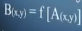
1 point operation

   features: the input image and output image are point-to-point copy operations. In this copy process, the gray value will be converted. This conversion operation can be linear or nonlinear. It can be expressed as:

   application: contrast enhancement, contrast stretching, image gray translation (brightening and darkening), binarization, edge line, cutting.

  case: linear point operation
   suppose an image Da, and obtain Da after linear point operation. The conversion function can be expressed as: Da=f(DA)=aDA+b
   A is the contrast adjustment parameter. If a > 1, the contrast will increase (the difference of gray value). If 0 < a < 1, the contrast will decrease. If a=1, the gray value will shift as a whole. If a < 0, the image gray level will be reversed.
   B is the gray value translation item. If b > 0, the image is brightened as a whole. If B < 0, the image is darkened as a whole.
  case: nonlinear point operation
   assuming that the image is very complex, it may not be an 8-bit image, but may be 12 bits or 16 bits. In this case, the pixel value of the image may be - 1000, + 1000. In this case, the computer may only want to focus on its positive range, so it is necessary to compress the whole gray value of the image, for example: f(x)=x+C (Dm-x)
   x is the gray value of the input image; C is the parameter controlling magnification and reduction, i.e. contrast coefficient; Dm is the maximum gray value parameter.
   x tends to the gray value pixel of the median, with obvious change; X tends to the pixels with gray values at both ends, and the change is relatively small.

2 algebraic (arithmetic) operations

   features: two (n) images, pixel to pixel operation to generate the third (n+1) image. And the size of the image should be consistent. It can be expressed as:

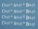
2.1 addition operation

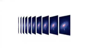
   (1) addition operation: ① remove noise by averaging. The reason for denoising is that the noise in nature exists in Random, and the noise can be removed by averaging multiple images. For example, through the high-power astronomical telescope + camera, the nebula in the night sky can be photographed, but these images are very unclear, because these high-power enlarged images introduce a lot of noise. The solution is to take many images continuously in a very short time, and then take the average of these images to get a clear image. ② Multiple exposures, one thing appears multiple times in the same image; ③ Blue screen photography, shooting under the blue screen, superimposing the background together.

  API: cv.add(img1, img2) function adds two images, or you can add two images through numpy operation, such as res=img1+img2
  note: there is a difference between opencv addition and numpy addition. The addition operation of OpenCV is saturation operation, while numpy adds modular operation.

import cv2
import matplotlib.pyplot as plt
import numpy as np
x=np.uint8([250])
y=np.uint8([10])
print(cv2.add(x,y))#250 + 10 = 260 saturation operation becomes 255
print(x+y)#250 + 10 = 260 mold taking operation becomes 4

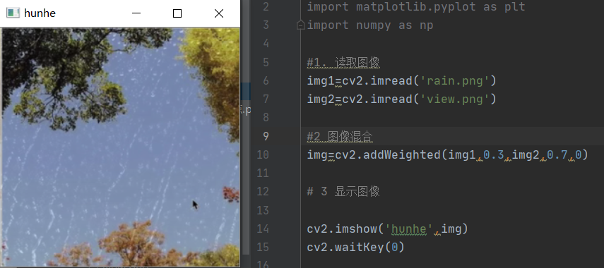
   image mixing is actually addition, but the difference is that the weights of the two images are different, giving people a feeling of mixing or transparency:
  g(x)=(1-α)f0(x)+aαf(x)
  API: cv2.addWeighted(img1,α，img2,β，γ)

import cv2
import matplotlib.pyplot as plt
import numpy as np

#1. Read image
img1=cv2.imread('rain.png')
img2=cv2.imread('view.png')

#2 image blending
img=cv2.addWeighted(img1,0.3,img2,0.7,0)

# 3 display image

cv2.imshow('hunhe',img)
cv2.waitKey(0)

2.2 subtraction operation

   (2) subtraction operation: ① remove the background through subtraction operation. For example, if the background is fixed and the foreground is a target moving, the background can be obtained and the background can be erased by subtraction; ② Target motion is detected by subtraction operation; ③ Seeking gradient is actually subtraction between pixels.

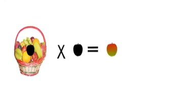
2.3 multiplication operation

   (3) multiplication operation: the algorithm has been able to obtain the optimal binarization value, binarize the image and obtain the region of interest (binary image), but the binary image has no pixel value information of the region of interest. Therefore, the multiplication operation can be applied to extract the pixel value information of the region of interest.

2.4 division operation

  (4) division operation

3 geometric operation

  target: change the spatial coordinate relationship of the image (translation, rotation...).
   geometric operation: it involves spatial conversion (described in detail in the registration part) and gray difference.

3.1 space conversion

3.1.1 translation transformation

   (1) translation

   definition: move the image to the corresponding position according to the specified direction and distance
  API: cv2.warpAffine(img,M,dsize)
   parameters:
     img: input image
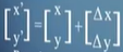
     M: 2 * 3 moving matrix
       for pixels at (x,y), set
       when it moves to (x+tx,y+ty), matrix M should be set as:

       M is a Numpy array of type np.float32.
     dsize: output image size
  note: the size of the output image should be in the form of (width, height). Remember, width = number of columns, height = number of rows

import cv2
import matplotlib.pyplot as plt
import numpy as np
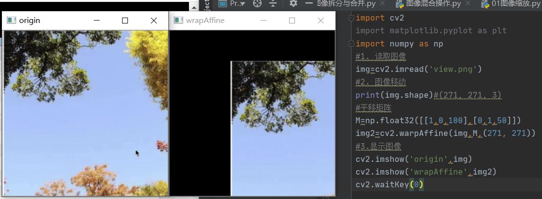
#1. Read image
img=cv2.imread('view.png')
#2. Image movement
print(img.shape)#(271, 271, 3)
#translation matrix 
M=np.float32([[1,0,100],[0,1,50]])
img2=cv2.warpAffine(img,M,(271, 271))

#3. Display image
cv2.imshow('origin',img)
cv2.imshow('wrapAffine',img2)
cv2.waitKey(0)

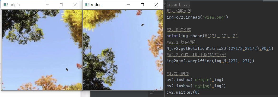
3.1.2 rotation transformation

   (2) rotation

   definition: image rotation refers to the process of rotating an image by a certain angle according to a certain position, and the image still maintains the original size during rotation. After image rotation, the horizontal symmetry axis, vertical symmetry axis and central coordinate origin of the image may be transformed, so the coordinates in image rotation need to be transformed accordingly.

  API:
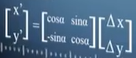
  M=cv2.getRotationMetrix2D(Center,angle,scale)
  cv2.warpAffine(img,M,dsize)
   parameters:
     Center: Center of rotation
     angle: rotation angle
     scale: scale

import cv2
import matplotlib.pyplot as plt
import numpy as np
#1. Read image
img=cv2.imread('view.png')

#2. Image rotation
print(img.shape)#(271, 271, 3)
##2.1 rotation matrix
M=cv2.getRotationMatrix2D((271/2,271/2),90,1)
##2.2 rotation is realized by using the API of translation
img2=cv2.warpAffine(img,M,(271, 271))

#3. Display image
cv2.imshow('origin',img)
cv2.imshow('rotion',img2)
cv2.waitKey(0)

3.1.3 scaling transformation

  (3) zoom

  definition: it is to adjust the size of the image, even if the image is enlarged or reduced
  API: cv2.resize(src,dsize,fx=0,fy=0,interpolation=cv2.INTER_LINEAR)
   parameters:
     src: input image
     dsize: absolute size, which directly specifies the size of the adjusted image
     fx,fy: relative size, set dsize to None, and then set fx,fy to scale factor.
  interpolation: difference method

interpolation	meaning
cv2.INTER_LINEAR	Bilinear difference
cv2.INTER_NEAREST	Nearest neighbor difference
cv2.INTER_AREA	Pixel area resampling, default
cv2.INTER_CUBIC	Bicubic interpolation

import cv2
import matplotlib.pyplot as plt
import numpy as np
#1. Read image
img=cv2.imread('view.png')
#2. Image scaling
#  2.1 absolute dimensions
img1=cv2.resize(img,(250,250),interpolation=cv2.INTER_LINEAR)
#  2.2 relative dimensions
img2=cv2.resize(img,dsize=None,fx=0.8,fy=0.6)

#3. Display image
cv2.imshow('origin',img)
cv2.imshow('juedui',img1)
cv2.imshow('xiangdui',img2)
cv2.waitKey(0)

   the results obtained by the operations of amplifying before rotating and rotating before amplifying are the same; The results obtained from the operations of zooming in first and zooming in first are inconsistent.

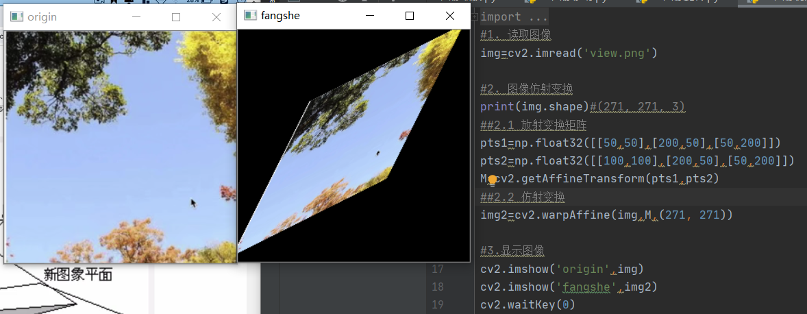
3.1.4 affine transformation

   definition: image affine transformation is a common function in deep learning preprocessing. Affine transformation is mainly a combination of image scaling, rotation, flipping and translation
  API:
  M=cv2.getAffineTransform(pts1,pts2)
  cv2.warpAffine(img,M,dsize)
   parameters:
     pts1: three points in the original drawing
     pts1: three points after transformation
  note: in affine transformation, all uneven lines in the original image are also parallel in the resulting image. In order to perform affine transformation, first find the three points in the original graph and the three points after affine transformation, and use these two groups of points and cv2.getAffineTransform() function to obtain 2 × Affine transformation matrix of 3; Then the affine transformation matrix is passed into the cv2.wrapAffine() function for affine transformation. The characteristic of affine transformation is that the relationship between points and lines is the same in the original graph, but the length of lines will change and the angle between lines will also change.

import cv2
import matplotlib.pyplot as plt
import numpy as np
#1. Read image
img=cv2.imread('view.png')

#2. Image affine transformation
print(img.shape)#(271, 271, 3)
##2.1 radiative transformation matrix
pts1=np.float32([[50,50],[200,50],[50,200]])
pts2=np.float32([[100,100],[200,50],[50,200]])
M=cv2.getAffineTransform(pts1,pts2)
##2.2 affine transformation
img2=cv2.warpAffine(img,M,(271, 271))

#3. Display image
cv2.imshow('origin',img)
cv2.imshow('fangshe',img2)
cv2.waitKey(0)

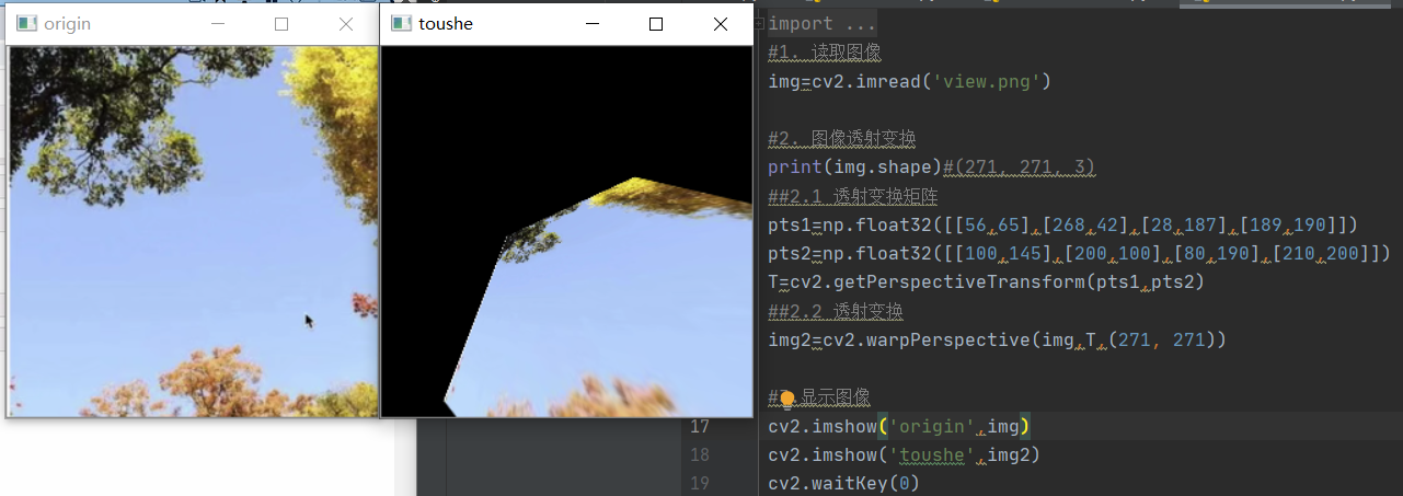
3.1.5 transmission transformation

   definition: transmission transformation is the result of viewing angle transformation. It refers to the transformation that uses the condition that the perspective center, image point and target point are collinear, rotates the background surface (perspective surface) around the trace (transmission axis) by a certain angle according to the perspective rotation law, destroys the original projection beam line, and can still keep the projection geometric image on the background surface unchanged.


  API:
  T=cv2.getPerspectiveTransform(pts1,pts2)
  cv2.warpPerspective(img,T,dsize)
   parameters:
     pts1: four points in the original drawing
     pts2: four points after transmission transformation
   note: in OpenCV, we need to find four points, of which any three are not collinear, and then obtain the transmission transformation matrix T through the four points and cv2.getPerspectiveTransform(), and use t for transmission transformation.

import cv2
import matplotlib.pyplot as plt
import numpy as np
#1. Read image
img=cv2.imread('view.png')

#2. Image transmission transformation
print(img.shape)#(271, 271, 3)
##2.1 transmission transformation matrix
pts1=np.float32([[56,65],[268,42],[28,187],[189,190]])
pts2=np.float32([[100,145],[200,100],[80,190],[210,200]])
T=cv2.getPerspectiveTransform(pts1,pts2)
##2.2 transmission transformation
img2=cv2.warpPerspective(img,T,(271, 271))

#3. Display image
cv2.imshow('origin',img)
cv2.imshow('toushe',img2)
cv2.waitKey(0)

3.2 image difference

   difference:
   (1) nearest neighbor difference: it is the copy of the gray value of the nearest point, but this method is not true and is prone to terrace effect.
   (2) linear difference: a square is formed between the difference point and the surrounding points. In the square, the weight is set according to the distance, and the gray value is calculated and superimposed as the gray value of the difference point.
   (3) bilinear difference