R language BUGS sequence Monte Carlo SMC, Markov transformation random volatility SV model, particle filter, METROPOLIS HASTINGS time series analysis

Keywords: Algorithm Machine Learning AI Deep Learning

Original link: http://tecdat.cn/?p=24162

In this example, we consider Markov transformation stochastic volatility model.

statistical model

Let yt be the dependent variable and xt be the unobserved logarithmic volatility of yt. For t ≤ tmax, the stochastic volatility model is defined as follows

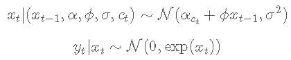
The state variable ct follows a two state Markov process with transition probability

N(m, σ 2) Represents the mean M And variance σ Normal distribution of 2.

BUGS language statistical model

File content ' vol.bug':

dlfie = 'vol.bug' #BUGS model file name

set up

Seed random number generator for repeatability

set.seed(0)

Load models and data

model parameter

dt = lst(t\_mx=t\_mx, sa=sima,
            alha=alpa, phi=pi, pi=pi, c0=c0, x0=x0)

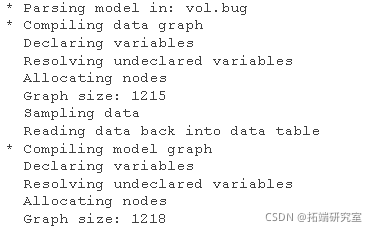
Parse and compile BUGS model and sample data

modl(mol\_le, ata,sl\_da=T)

Draw data

plot(1:tmx, y, tpe='l',xx = 'n')

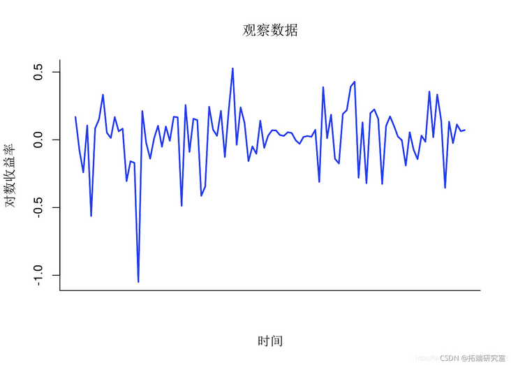
Logarithmic rate of return

Sequential Monte Carlo_ Sequential Monte Carlo_

function

n= 5000 #  Number of particles
var= c('x') #  Variables to monitor
out = smc(moe, vra, n)

Model diagnosis

diagnosis(out)

Drawing smoothing ESS

plt(ess, tpe='l')
lins(1:ta, ep(0,tmx))

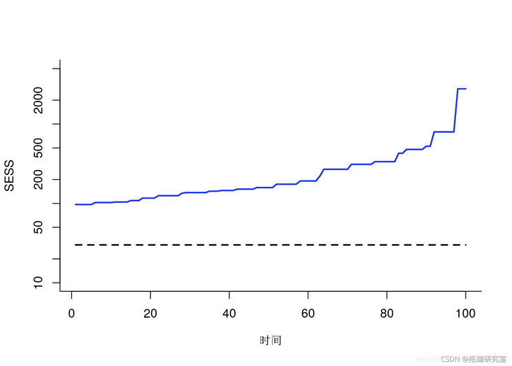
SMC: SESS

Paint weighted particles

plt(1:tax, out,)
for (t in 1:_ax) {
  vl = uiq(valest,\])
  wit = sply(vl, UN=(x) {
    id = utm$$sles\[t,\] == x
    rtrn(sm(wiht\[t,ind\]))
  })
  pints(va)
}
lies(1t_x, at$xue)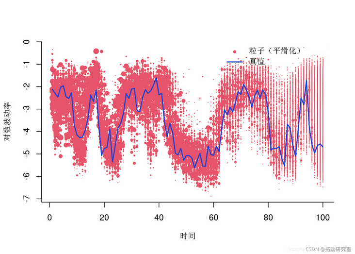

Particles (smooth)

Summary statistics

summary(out)

Mapping filter estimation

men = mean
qan = quant

x = c(1:tmx, _a:1)
y = c(fnt, ev(x__qat))
plot(x, y)
pln(x, y, col)
lines(1:tma,x_ean)

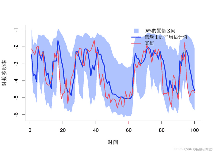
Filter estimation

Mapping smoothing estimation

plt(x,y, type='')

polgon(x, y)
lins(1:tmx, mean)

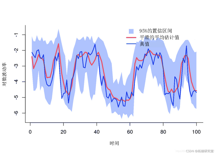
Smoothing estimation

Edge filtering and smoothing density

denty(out)
indx = c(5, 10, 15)

for (k in 1:legh) {
  inex
  plt(x)
  pints(xtrue\[k\])
}

Marginal posterior

Particle independent metropolis Hastings

function

mh = mit(mol, vre)

mh(bm, brn, prt) #  Pre burn iteration

mh(bh, ni, n_at, hn=tn) #  Return sample

Some summary statistics

smay(otmh, pro=c(.025, .975))

Posterior mean and quantile

mean
quant
plot(x, y)

polo(x, y, border=NA)
lis(1:tax, mean)

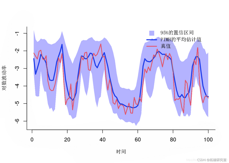
Posterior mean and quantile

Trace map of MCMC samples

for (k in 1:length {
  tk = idx\[k\]
  plot(out\[tk,\]
    )
  points(0, xtetk)
}

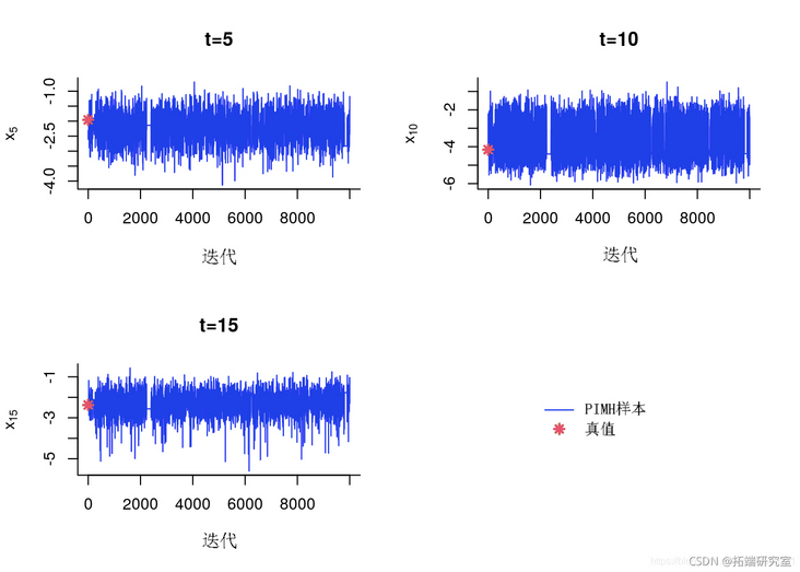
Tracking sample

A posteriori histogram

for (k in 1:lngh) {
  k = inex\[k\]
  hit(mh$x\[t,\])
  poits(true\[t\])
}

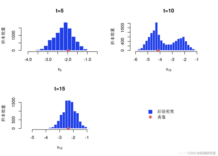
Back edge histogram

A posteriori kernel density estimation

for (k in 1:lnth(ie)) {
 idx\[k\]
  desty(out\[t,\])
  plt(eim)
  poit(xtu\[t\])
}

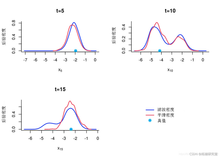
KDE posterior edge estimation

sensitivity analysis

We want to study the parameters α Value sensitivity

Algorithm parameters

nr = 50 #  Number of particles
gd <- seq(-5,2,.2) #  A numerical grid of components
A = rep(grd, tes=leg) #  Value of the first component
B = rep(grd, eah=lnh) #  Value of the second component
vaue = ist('lph' = rid(A, B))

Operational Sensitivity Analysis

sny(oel,aaval, ar)

Plot LOG edge likelihood and penalty LOG edge likelihood

#  Avoid standardization problems through threshold processing
thr = -40
z = atx(mx(thr, utike), row=enth(rd))

plot(z, row=grd, col=grd,
          at=sq(thr))

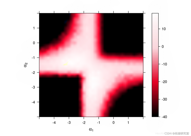
Sensitivity: log likelihood

Programmer Group