1, Introduction to LDA and SVM
- Linear Discriminant Analysis (LDA) is a classical supervised data dimensionality reduction method. The main idea of LDA is to project the data in a high-dimensional space into a low-dimensional space, and after the projection, it is necessary to ensure that the intra class variance of each category is small and the mean difference between categories is large, which means that after the high-dimensional data of the same category are projected into a low-dimensional space, the same categories gather together, but the different categories are far apart.
- In machine learning, support vector machine (SVM) is a supervised learning model with related learning algorithms, which analyzes the data used for classification and regression analysis. Given a set of training examples, each example is marked as belonging to one or the other of the two categories, the SVM training algorithm constructs a model, assigns the new example to one category or the other category, and makes it a non probabilistic binary linear classifier. The SVM model represents the examples as points in space, and the mapping makes the examples of individual categories divided by the explicit gap as wide as possible. Then map the new examples to the same space and predict which edge they belong to a category.
2, LDA implementation code
- Import the package you want to use
from sklearn.discriminant_analysis import LinearDiscriminantAnalysis as lda#Import LDA Algorithm
from sklearn.datasets._samples_generator import make_classification #Import classification builder
import matplotlib.pyplot as plt #Import tools for drawing
import numpy as np
import pandas as pd
- Get the data set and train with the make imported above_ The classification function obtains the dataset
x,y=make_classification(n_samples=500,n_features=2,n_redundant=0,n_classes=2,n_informative=1,n_clusters_per_class=1,class_sep=0.5,random_state=100)
"""
n_features :Number of features= n_informative() + n_redundant + n_repeated
n_informative: Number of multi information features
n_redundant: Redundant information, informative Random linear combination of features
n_repeated : Duplicate information, random extraction n_informative and n_redundant features
n_classes: Classification category
n_clusters_per_class : A category consists of several cluster Constitutive

"""
plt.scatter(x[:,0],x[:,1], marker='o', c=y)
plt.show()
x_train=x[:60, :60]
y_train=y[:60]
x_test=x[40:, :]
y_test=y[40:]
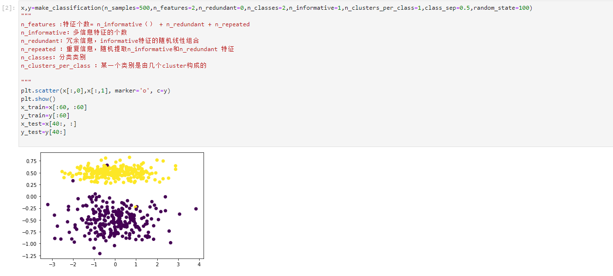
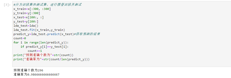
- The data set is divided into training set and test set, and the classification ratio is 6:4. After training, the accuracy is obtained by using the test set
#It is divided into training set and test set for model training and testing
x_train=x[:300, :300]
y_train=y[:300]
x_test=x[200:, :]
y_test=y[200:]
lda_test=lda()
lda_test.fit(x_train,y_train)
predict_y=lda_test.predict(x_test)#Get predicted results
count=0
for i in range(len(predict_y)):
    if predict_y[i]==y_test[i]:
        count+=1
print("The number of accurate forecasts is"+str(count))
print("The accuracy is"+str(count/len(predict_y)))
3, SVM dataset for visual classification
1. Linear kernel
- Import package
# Importing moon dataset and svm method
#This is linear svm
from sklearn import datasets #Import dataset
from sklearn.svm import LinearSVC #Import linear svm
from matplotlib.colors import ListedColormap
from sklearn.preprocessing import StandardScaler
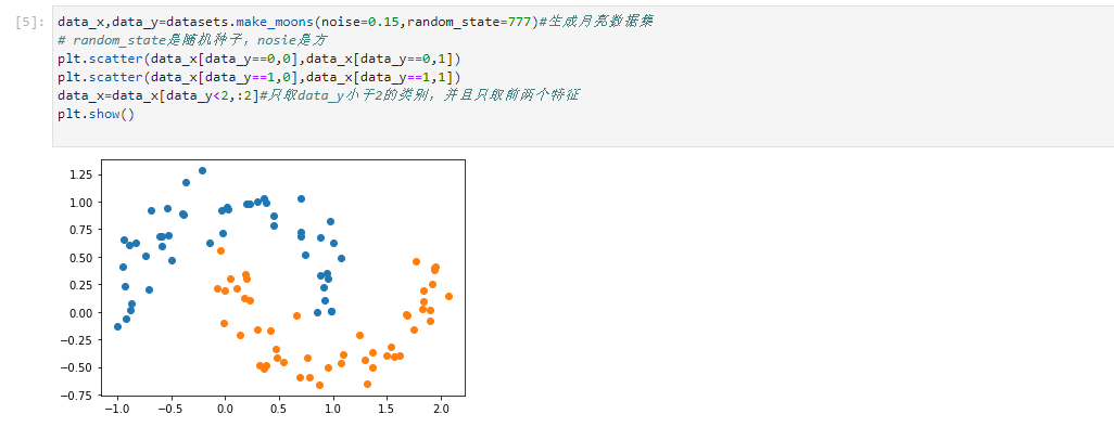
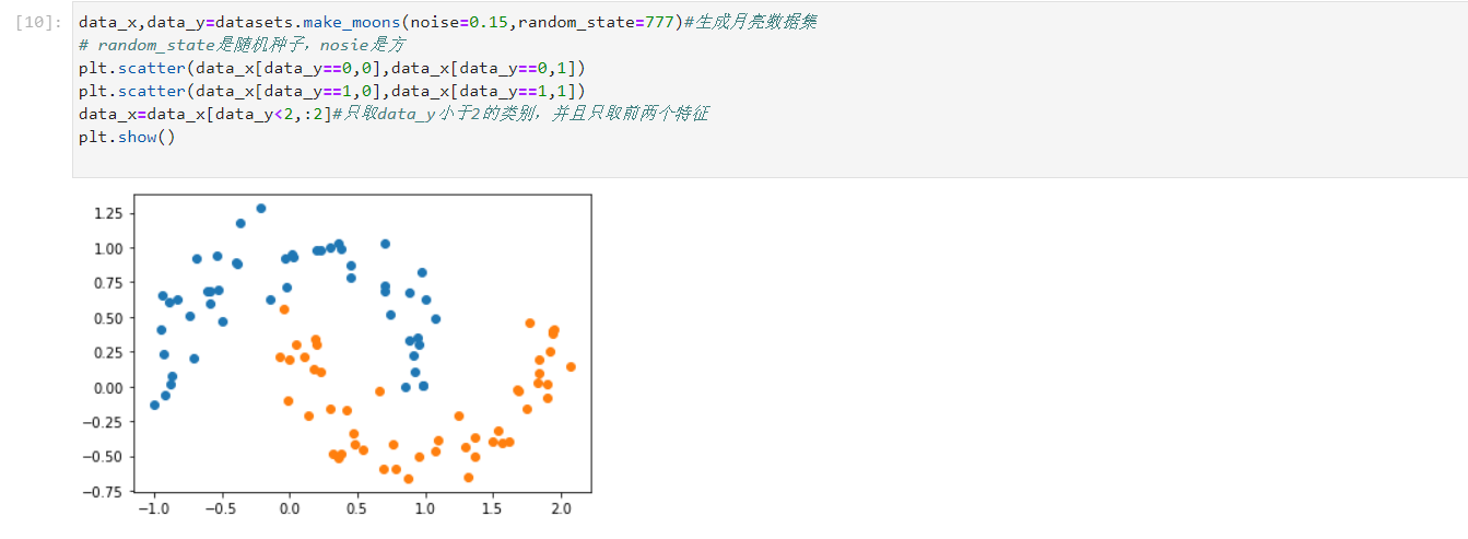
- Obtain data
data_x,data_y=datasets.make_moons(noise=0.15,random_state=777)#Generate moon dataset
# random_state is a random seed and nosie is a square
plt.scatter(data_x[data_y==0,0],data_x[data_y==0,1])
plt.scatter(data_x[data_y==1,0],data_x[data_y==1,1])
data_x=data_x[data_y<2,:2]#Data only_ Y is less than 2, and only the first two features are taken
plt.show()
- Standardize and train data
scaler=StandardScaler()# Standardization
scaler.fit(data_x)#Calculate the mean and variance of training data
data_x=scaler.transform(data_x) #Then use the mean and variance in scaler to convert X and standardize X
liner_svc=LinearSVC(C=1e9,max_iter=100000)#For linear svm classifier, iter is the number of iterations, and the value of c determines the fault tolerance. The larger c is, the smaller the fault tolerance is
liner_svc.fit(data_x,data_y)
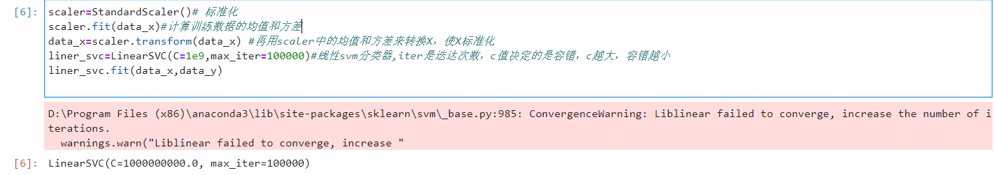
As shown in the figure, there will be warnings, but there are still results. Ignore the warnings.
- Write a boundary drawing function to prepare for the following visual classification
# Boundary drawing function
def plot_decision_boundary(model,axis):
    x0,x1=np.meshgrid(
        np.linspace(axis[0],axis[1],int((axis[1]-axis[0])*100)).reshape(-1,1),
        np.linspace(axis[2],axis[3],int((axis[3]-axis[2])*100)).reshape(-1,1))
    # The meshgrid function returns a coordinate matrix from a coordinate vector
    x_new=np.c_[x0.ravel(),x1.ravel()]
    y_predict=model.predict(x_new)#Get predicted value
    zz=y_predict.reshape(x0.shape)
    custom_cmap=ListedColormap(['#EF9A9A','#FFF59D','#90CAF9'])
    plt.contourf(x0,x1,zz,cmap=custom_cmap)
- Drawing and output parameter weight and model intercept
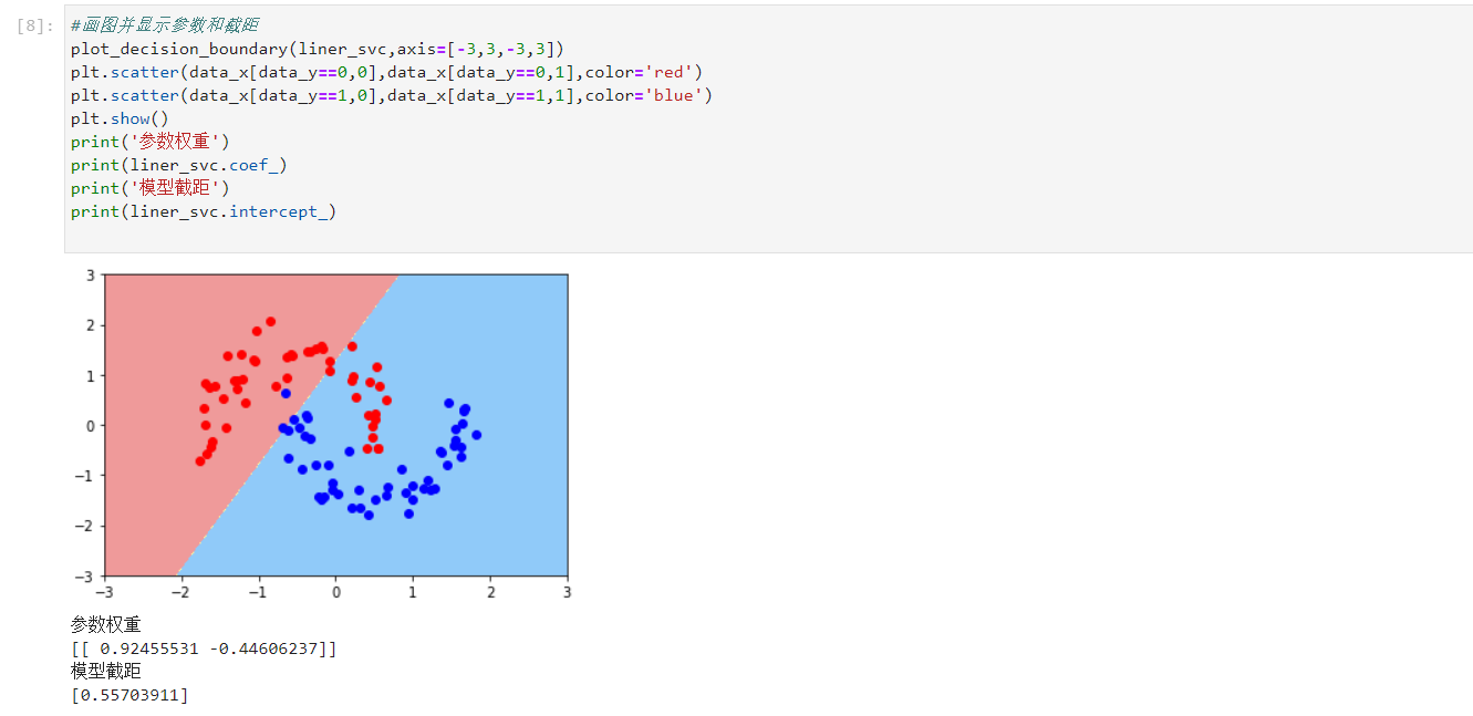
#Draw and display parameters and intercept
plot_decision_boundary(liner_svc,axis=[-3,3,-3,3])
plt.scatter(data_x[data_y==0,0],data_x[data_y==0,1],color='red')
plt.scatter(data_x[data_y==1,0],data_x[data_y==1,1],color='blue')
plt.show()
print('Parameter weight')
print(liner_svc.coef_)
print('Model intercept')
print(liner_svc.intercept_)
2. Polynomial kernel
- Import package with pipeline kernel polynomial regression
#This is polynomial kernel svm
from sklearn import datasets #Import dataset
from sklearn.svm import LinearSVC #Import linear svm
from sklearn.pipeline import Pipeline #Import pipes in python
from matplotlib.colors import ListedColormap
import matplotlib.pyplot as plt
from sklearn.preprocessing import StandardScaler,PolynomialFeatures #Import polynomial regression and standardization
- The generated data, which is also the moon data set, is consistent with linear svm
data_x,data_y=datasets.make_moons(noise=0.15,random_state=777)#Generate moon dataset
# random_state is a random seed and nosie is a square
plt.scatter(data_x[data_y==0,0],data_x[data_y==0,1])
plt.scatter(data_x[data_y==1,0],data_x[data_y==1,1])
data_x=data_x[data_y<2,:2]#Data only_ Y is less than 2, and only the first two features are taken
plt.show()
- pipeline is used for integrated programming. For convenience, it is put into the function
 def PolynomialSVC(degree,c=10):#Polynomial svm
    return Pipeline([
            # Mapping source data to third-order polynomials
            ("poly_features", PolynomialFeatures(degree=degree)),
            # Standardization
            ("scaler", StandardScaler()),
            # SVC linear classifier
            ("svm_clf", LinearSVC(C=10, loss="hinge", random_state=42,max_iter=10000))
        ])
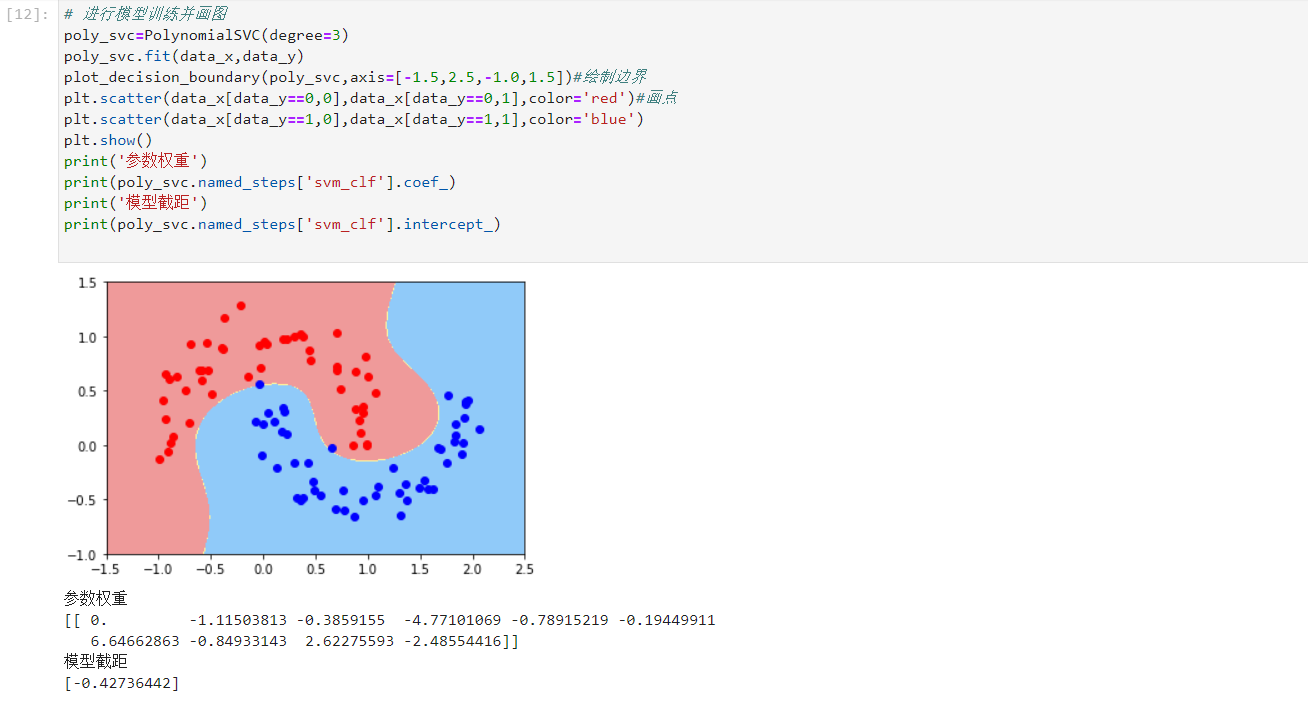
- Model training and drawing
# Model training and drawing
poly_svc=PolynomialSVC(degree=3)
poly_svc.fit(data_x,data_y)
plot_decision_boundary(poly_svc,axis=[-1.5,2.5,-1.0,1.5])#Draw boundary
plt.scatter(data_x[data_y==0,0],data_x[data_y==0,1],color='red')#Draw point
plt.scatter(data_x[data_y==1,0],data_x[data_y==1,1],color='blue')
plt.show()
print('Parameter weight')
print(poly_svc.named_steps['svm_clf'].coef_)
print('Model intercept')
print(poly_svc.named_steps['svm_clf'].intercept_)
3. Gaussian kernel
- Import package
## Import package
from sklearn import datasets #Import dataset
from sklearn.svm import SVC #Import svm
from sklearn.pipeline import Pipeline #Import pipes in python
import matplotlib.pyplot as plt
from sklearn.preprocessing import StandardScaler#Import standardization
- Define SVM Gaussian model
def RBFKernelSVC(gamma=1.0):
    return Pipeline([
        ('std_scaler',StandardScaler()),
        ('svc',SVC(kernel='rbf',gamma=gamma))
    ])
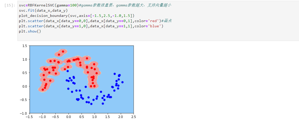
- Carry out model training and draw graphics. The gamma parameter is also very important. The larger the gamma parameter is, the smaller the support vector is, which is similar to C. changing the gamma value will change the judgment area
svc=RBFKernelSVC(gamma=100)#Gamma parameter is very important. The larger the gamma parameter, the smaller the support vector
svc.fit(data_x,data_y)
plot_decision_boundary(svc,axis=[-1.5,2.5,-1.0,1.5])
plt.scatter(data_x[data_y==0,0],data_x[data_y==0,1],color='red')#Draw point
plt.scatter(data_x[data_y==1,0],data_x[data_y==1,1],color='blue')
plt.show()
4, Summary
We have a preliminary understanding and practice of LDA and SVM, and our understanding of the role is a little deeper than before. LDA projects all points onto a straight line, and then looks for a classified straight line. SVM calculates the support vector near the boundary and confirms the boundary through the support vector. The understanding of the principle is still quite shallow, and we need to deepen the study of the principle