1 Introduction to the experiment

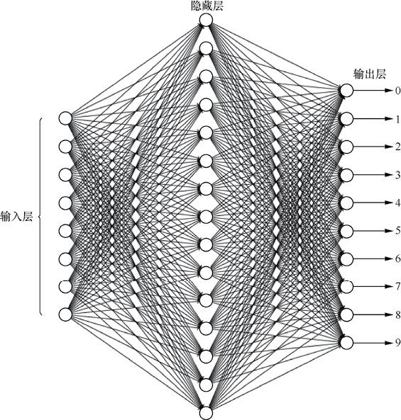
Experimental requirements: implement a handwritten numeral recognition program, as shown in the figure below. The neural network is required to include a hidden layer, and the number of neurons in the hidden layer is 15.

Overall idea: mainly refer to the introduction of neural network in Chapter 5 of watermelon book, and use batch gradient descent to train neural network.

Tip: the overall code and data set are linked at the end of the paper

2 read and process data

Data reading idea:

• The image given in the data set is a 28 * 28 gray image. After reading the image by plt.imread() function, it is a 28x28 array. If we use neural network for training, we can treat each pixel as a feature, so we use numpy.reshape method to turn the image into a 1x784 array. Read all the data and add it into the data set data, and add the corresponding labels into labels in the same order.
• Then use the np.random.permutation method to disrupt the index and use the proportion of the incoming test data_ Ratio divides the data into test set and training set.
• The mean and standard deviation of training samples are used to standardize the training data and test data. Standardization is very important. It began to ignore the links of standardization, and the accuracy of neural network has not achieved the effect.
• Return dataset

This part of the code is as follows:

# Read picture data parameters: proportion of data path test set
def loadImageData(trainingDirName='data/', test_ratio=0.3):
    from os import listdir
    data = np.empty(shape=(0, 784))
    labels = np.empty(shape=(0, 1))

    for num in range(10):
        dirName = trainingDirName + '%s/' % (num)  # Gets the current digital file path
        # print(listdir(dirName))
        nowNumList = [i for i in listdir(dirName) if i[-3:] == 'bmp']  # Get the picture file inside
        labels = np.append(labels, np.full(shape=(len(nowNumList), 1), fill_value=num), axis=0)  # Add picture labels
        for aNumDir in nowNumList:  # Read each picture into
            imageDir = dirName + aNumDir  # Construct picture path
            image = plt.imread(imageDir).reshape((1, 784))  # Read picture data
            data = np.append(data, image, axis=0)  
    # Partition dataset
    m = data.shape[0]
    shuffled_indices = np.random.permutation(m)  # Scramble data
    test_set_size = int(m * test_ratio)
    test_indices = shuffled_indices[:test_set_size]
    train_indices = shuffled_indices[test_set_size:]

    trainData = data[train_indices]
    trainLabels = labels[train_indices]

    testData = data[test_indices]
    testLabels = labels[test_indices]

    # The training samples and test samples are normalized by using the unified mean standard deviation
    tmean = np.mean(trainData)
    tstd = np.std(testData)

    trainData = (trainData - tmean) / tstd
    testData = (testData - tmean) / tstd
    return trainData, trainLabels, testData, testLabels

**OneHot coding: * * due to the characteristics of neural network, when performing multi classification tasks, the output of each neuron corresponds to a class, so the label of each training sample is transformed into OneHot form (map the data of 0-9 into a vector with length of 10, the value of the corresponding position of each sample is 1, and the rest is 0).

# OneHot encode the output label parameter: labels label to be encoded_ Number of class codes
def OneHotEncoder(labels,Label_class):
    one_hot_label = np.array([[int(i == int(labels[j])) for i in range(Label_class)] for j in range(len(labels))])
    return one_hot_label

3 training neural network

Activation function: the sigmoid function is used as the activation function, but the overflow warning always appears in the training process when using the definition. Therefore, the function is transformed in the following form.

# sigmoid activation function
def sigmoid(z):
    for r in range(z.shape[0]):
        for c in range(z.shape[1]):
            if z[r,c] >= 0:
                z[r,c] = 1 / (1 + np.exp(-z[r,c]))
            else :
                z[r,c] = np.exp(z[r,c]) / (1 + np.exp(z[r,c]))
    return z

Loss function: use the mean square error loss function. In fact, I feel that it is also possible to directly use the prediction accuracy in this topic.

def cost(prediction, labels):
    return np.mean(np.power(prediction - labels,2))

**Training: * * finally came to the tense and exciting training session. The neural network obtains the output of the network from the input layer through the output layer of the hidden layer, which is called forward propagation, and the process of adjusting the weight and bias from the output layer according to the gradient descent method is called back propagation.

Forward propagation multiplies the output value of each node by the corresponding weight between each layer ω \omega ω (omega1 omega2 in the corresponding function) is transmitted to the node of the next layer. The node of the next layer sums all the data transmitted from the previous layer and subtracts the offset theta (at this time, h_in o_in in the data corresponding function). Finally, the next layer (h_out o_out in the corresponding function) is output by activating the function.

After the forward propagation is completed, a loss is calculated for later analysis.

Back propagation uses gradient descent method to update the weight and bias. Here is the most important part. According to the watermelon book, it can be deduced that the adjustment amount of the weight of the output layer is η y i ^ ( 1 − y i ^ ) ( y i − y i ^ ) b h \eta\hat{y_i}(1-\hat{y_i})(y_i - \hat{y_i})b_h η yi ^ (1 − yi ^) (yi − yi ^) bh, where η \eta η For learning rate, y i   y i ^ y_i \space\hat{y_i} yi​   Yi ^ is the real value of the corresponding data and the output of the network, b h b_h bh ＾ is the output value of the hidden layer. Another important point here is that if the formula is vectorized, we need to focus on the shape of the output matrix and the relationship between each matrix data. d2 in the code corresponds to d2 in the formula y i ^ ( 1 − y i ^ ) ( y i − y i ^ ) \hat{y_i}(1-\hat{y_i})(y_i - \hat{y_i}) For the part of yi ^ (1 − yi ^) (yi − yi ^), you need to multiply the corresponding values. Finally, this part and b h b_h bh ， perform matrix multiplication and multiply the learning rate η \eta η Get the weight adjustment quantity and add it to the weight (except for the number of training set samples m in the code, because the product of d2 and h_out accumulates all training samples, so it is necessary to calculate the average).

The adjustment methods of other weights and offsets are similar to this. I don't introduce them too much (in fact, I have to go to class tomorrow. I have to go to bed too late. I'll make up here and other unspecified places when I'm free). See watermelon book for details.

# Training round ANN parameters: training data label input layer hidden layer output layer size input layer hidden layer connection weight hidden layer output layer connection weight offset 1 offset 2 learning rate
def trainANN(X, y, input_size, hidden_size, output_size, omega1, omega2, theta1, theta2, learningRate):
    # Number of samples obtained
    m = X.shape[0]
    # Convert matrix X,y into numpy matrix
    X = np.matrix(X)
    y = np.matrix(y)

    # Forward propagation calculates the output of each layer
    # Hidden layer input shape=m*hidden_size
    h_in = np.matmul(X, omega1.T) - theta1.T
    # Hidden layer output shape=m*hidden_size
    h_out = sigmoid(h_in)
    # Input shape of output layer = m * output_ size
    o_in = np.matmul(h_out, omega2.T) - theta2.T
    # Output shape of output layer = m * output_ size
    o_out = sigmoid(o_in)

    # Current loss
    all_cost = cost(o_out, y)

    # Back propagation
    # Output layer parameter update
    d2 = np.multiply(np.multiply(o_out, (1 - o_out)), (y - o_out))
    omega2 += learningRate * np.matmul(d2.T, h_out) / m
    theta2 -= learningRate * np.sum(d2.T, axis=1) / m

    # Hidden layer parameter update
    d1 = np.multiply(h_out, (1 - h_out))
    omega1 += learningRate * (np.matmul(np.multiply(d1, np.matmul(d2, omega2)).T, X) / float(m))
    theta1 -= learningRate * (np.sum(np.multiply(d1, np.matmul(d2, omega2)).T, axis=1) / float(m))

    return omega1, omega2, theta1, theta2, all_cost

4 network test

Prediction function: it is relatively simple here. The forward propagation part is the same as before. Because the final network output is the sample and x is the probability of each class, it is only necessary to use np.argmax function to calculate the subscript with the largest probability value, and the subscript 0-9 exactly corresponds to the value of the number.

# Data prediction
def predictionANN(X, omega1, omega2, theta1, theta2):
    # Number of samples obtained
    m = X.shape[0]
    # Convert matrix X,y into numpy matrix
    X = np.matrix(X)

    # Forward propagation calculates the output of each layer
    # Hidden layer input shape=m*hidden_size
    h_in = np.matmul(X, omega1.T) - theta1.T
    # Hidden layer output shape=m*hidden_size
    h_out = sigmoid(h_in)
    # Input shape of output layer = m * output_ size
    o_in = np.matmul(h_out, omega2.T) - theta2.T
    # Output shape of output layer = m * output_ size
    o_out = np.argmax(sigmoid(o_in), axis=1)

    return o_out

Accuracy calculation: all test data X are predicted here, and the accuracy is calculated by calculating the average value of the number of predicted labels y-hat consistent with the real labels y.

# Calculation model accuracy
def computeAcc(X, y, omega1, omega2, theta1, theta2):
    y_hat = predictionANN(X,omega1, omega2,theta1,theta2)
    return np.mean(y_hat == y)

Main function: in the main function, call the above function to predict the accuracy of network training, and use loss_list acc_list two lists save the accuracy and error of each round in the training process, using acc_max tracks the model with the maximum accuracy, and uses pickle to save the model (actually the parameters of the neural network), which can be read later. I will also lose when the training is finished_ list acc_ The list is saved (the idea is that you can use the training data to make a good picture). The last part draws the trend of loss and accuracy with the number of training times. The results are as follows:

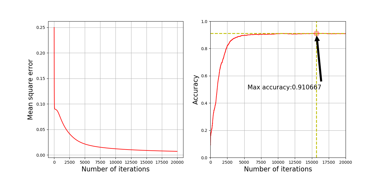
It can be seen that the model just ran through, and the effect is not good. After training for several hours, the accuracy rate is only 91%. The reason may be that the model is not regularized and the learning rate is not dynamically adjusted.

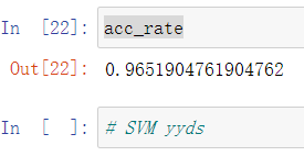
On the contrary, the accuracy of SVM model can easily reach more than 97%.

# get data
from sklearn.datasets import fetch_openml
from sklearn.svm import SVC
mnist = fetch_openml('mnist_784', version=1, as_frame=False) # DF type of Pandas is returned by default
# The dataset loaded by sklearn is similar to the dictionary structure
from sklearn.preprocessing import StandardScaler
X, y = mnist["data"], mnist["target"]
stder = StandardScaler() 
X = stder.fit_transform(X)
# Dividing training set and test set
test_ratio = 0.3

shuffled_indices = np.random.permutation(X.shape[0]) # Scramble data
test_set_size = int(X.shape[0] * test_ratio)
test_indices = shuffled_indices[:test_set_size]
train_indices = shuffled_indices[test_set_size:]

X_train, X_test, y_train, y_test = X[train_indices], X[test_indices], y[train_indices], y[test_indices]
# Training SVM

cls_svm = SVC(C=1.0, kernel='rbf')
cls_svm.fit(X_train,y_train)
y_pre = cls_svm.predict(X_test)
acc_rate = np.sum(y_pre == y_test) / float(y_pre.shape[0])
acc_rate

Shiver~~~

Finally, paste all codes:

import numpy as np
import matplotlib.pyplot as plt
import pickle

# Read picture data
def loadImageData(trainingDirName='data/', test_ratio=0.3):
    from os import listdir
    data = np.empty(shape=(0, 784))
    labels = np.empty(shape=(0, 1))

    for num in range(10):
        dirName = trainingDirName + '%s/' % (num)  # Gets the current digital file path
        # print(listdir(dirName))
        nowNumList = [i for i in listdir(dirName) if i[-3:] == 'bmp']  # Get the picture file inside
        labels = np.append(labels, np.full(shape=(len(nowNumList), 1), fill_value=num), axis=0)  # Add picture labels
        for aNumDir in nowNumList:  # Read each picture into
            imageDir = dirName + aNumDir  # Construct picture path
            image = plt.imread(imageDir).reshape((1, 784))  # Read picture data
            data = np.append(data, image, axis=0)  
    # Partition dataset
    m = data.shape[0]
    shuffled_indices = np.random.permutation(m)  # Scramble data
    test_set_size = int(m * test_ratio)
    test_indices = shuffled_indices[:test_set_size]
    train_indices = shuffled_indices[test_set_size:]

    trainData = data[train_indices]
    trainLabels = labels[train_indices]

    testData = data[test_indices]
    testLabels = labels[test_indices]

    # The training samples and test samples are normalized by using the unified mean standard deviation
    tmean = np.mean(trainData)
    tstd = np.std(testData)

    trainData = (trainData - tmean) / tstd
    testData = (testData - tmean) / tstd
    return trainData, trainLabels, testData, testLabels

# OneHot encodes the output tag
def OneHotEncoder(labels,Label_class):
    one_hot_label = np.array([[int(i == int(labels[j])) for i in range(Label_class)] for j in range(len(labels))])
    return one_hot_label

# sigmoid activation function
def sigmoid(z):
    for r in range(z.shape[0]):
        for c in range(z.shape[1]):
            if z[r,c] >= 0:
                z[r,c] = 1 / (1 + np.exp(-z[r,c]))
            else :
                z[r,c] = np.exp(z[r,c]) / (1 + np.exp(z[r,c]))
    return z

# Calculated mean square error parameter: predicted value, true value
def cost(prediction, labels):
    return np.mean(np.power(prediction - labels,2))


# Training round ANN parameters: training data label input layer hidden layer output layer size input layer hidden layer connection weight hidden layer output layer connection weight offset 1 offset 2 learning rate
def trainANN(X, y, input_size, hidden_size, output_size, omega1, omega2, theta1, theta2, learningRate):
    # Number of samples obtained
    m = X.shape[0]
    # Convert matrix X,y into numpy matrix
    X = np.matrix(X)
    y = np.matrix(y)

    # Forward propagation calculates the output of each layer
    # Hidden layer input shape=m*hidden_size
    h_in = np.matmul(X, omega1.T) - theta1.T
    # Hidden layer output shape=m*hidden_size
    h_out = sigmoid(h_in)
    # Input shape of output layer = m * output_ size
    o_in = np.matmul(h_out, omega2.T) - theta2.T
    # Output shape of output layer = m * output_ size
    o_out = sigmoid(o_in)

    # Current loss
    all_cost = cost(o_out, y)

    # Back propagation
    # Output layer parameter update
    d2 = np.multiply(np.multiply(o_out, (1 - o_out)), (y - o_out))
    omega2 += learningRate * np.matmul(d2.T, h_out) / m
    theta2 -= learningRate * np.sum(d2.T, axis=1) / m

    # Hidden layer parameter update
    d1 = np.multiply(h_out, (1 - h_out))
    omega1 += learningRate * (np.matmul(np.multiply(d1, np.matmul(d2, omega2)).T, X) / float(m))
    theta1 -= learningRate * (np.sum(np.multiply(d1, np.matmul(d2, omega2)).T, axis=1) / float(m))

    return omega1, omega2, theta1, theta2, all_cost


# Data prediction
def predictionANN(X, omega1, omega2, theta1, theta2):
    # Number of samples obtained
    m = X.shape[0]
    # Convert matrix X,y into numpy matrix
    X = np.matrix(X)

    # Forward propagation calculates the output of each layer
    # Hidden layer input shape=m*hidden_size
    h_in = np.matmul(X, omega1.T) - theta1.T
    # Hidden layer output shape=m*hidden_size
    h_out = sigmoid(h_in)
    # Input shape of output layer = m * output_ size
    o_in = np.matmul(h_out, omega2.T) - theta2.T
    # Output shape of output layer = m * output_ size
    o_out = np.argmax(sigmoid(o_in), axis=1)

    return o_out


# Calculation model accuracy
def computeAcc(X, y, omega1, omega2, theta1, theta2):
    y_hat = predictionANN(X,omega1, omega2,theta1,theta2)
    return np.mean(y_hat == y)


if __name__ == '__main__':
    # Load model data
    trainData, trainLabels, testData, testLabels = loadImageData()

    # Initialization settings
    input_size = 784
    hidden_size = 15
    output_size = 10
    lamda = 1

    # Random initialization of network parameters
    omega1 = np.matrix((np.random.random(size=(hidden_size,input_size)) - 0.5) * 0.25) # 15*784
    omega2 = np.matrix((np.random.random(size=(output_size,hidden_size)) - 0.5) * 0.25)  # 10*15

    # Initialize two offsets
    theta1 = np.matrix((np.random.random(size=(hidden_size,1)) - 0.5) * 0.25) # 15*1
    theta2 = np.matrix((np.random.random(size=(output_size,1)) - 0.5) * 0.25) # 10*1
    # Learning rate
    learningRate = 0.1
    # data set
    m = trainData.shape[0] # Number of samples
    X = np.matrix(trainData) # Input data m*784
    y_onehot=OneHotEncoder(trainLabels,10) # Label m*10

    iters_num = 20000  # Sets the number of cycles
    loss_list = []
    acc_list = []
    acc_max = 0.0  # Maximum accuracy saves the model when the accuracy reaches the maximum
    acc_max_iters = 0

    for i in range(iters_num):
        omega1, omega2, theta1, theta2, loss = trainANN(X, y_onehot, input_size, hidden_size, output_size, omega1,
                                                        omega2, theta1, theta2, learningRate)
        loss_list.append(loss)
        acc_now = computeAcc(testData, testLabels, omega1, omega2, theta1, theta2)  # Calculation accuracy
        acc_list.append(acc_now)
        if acc_now > acc_max:  # If the accuracy reaches the maximum, save the model
            acc_max = acc_now
            acc_max_iters = i  # Save the coordinates for easy marking on the drawing
            # Save model parameters
            f = open(r"./best_model", 'wb')
            pickle.dump((omega1, omega2, theta1, theta2), f, 0)
            f.close()
        if i % 100 == 0:  # Print the accuracy information every 100 training rounds
            print("%d  Now accuracy : %f"%(i,acc_now))

    # Save training data for analysis
    f = open(r"./loss_list", 'wb')
    pickle.dump(loss_list, f, 0)
    f.close()

    f = open(r"./acc_list", 'wb')
    pickle.dump(loss_list, f, 0)
    f.close()

    # Drawing graphics
    plt.figure(figsize=(13, 6))
    plt.subplot(121)
    x1 = np.arange(len(loss_list))
    plt.plot(x1, loss_list, "r")
    plt.xlabel(r"Number of iterations", fontsize=16)
    plt.ylabel(r"Mean square error", fontsize=16)
    plt.grid(True, which='both')

    plt.subplot(122)
    x2 = np.arange(len(acc_list))
    plt.plot(x2, acc_list, "r")
    plt.xlabel(r"Number of iterations", fontsize=16)
    plt.ylabel(r"Accuracy", fontsize=16)
    plt.grid(True, which='both')
    plt.annotate('Max accuracy:%f' % (acc_max),  # Dimension maximum precision value
                 xy=(acc_max_iters, acc_max),
                 xytext=(acc_max_iters * 0.7, 0.5),
                 arrowprops=dict(facecolor='black', shrink=0.05),
                 ha="center",
                 fontsize=15,
                 )
    plt.plot(np.linspace(acc_max_iters, acc_max_iters, 200), np.linspace(0, 1, 200), "y--", linewidth=2, )  # Maximum precision iterations
    plt.plot(np.linspace(0, len(acc_list), 200), np.linspace(acc_max, acc_max, 200), "y--", linewidth=2)  # Maximum accuracy

    plt.scatter(acc_max_iters, acc_max, s=180, facecolors='#FFAAAA')  # Dimension maximum precision point
    plt.axis([0, len(acc_list), 0, 1.0])  # Set coordinate range
    plt.savefig("ANN_plot")  # Save picture
    plt.show()

Code and dataset network disk connection:

Link: https://pan.baidu.com/s/1kGJtaylhyUmkzOmWvovi1A
Extraction code: 4zpb

In fact, it was the homework assigned by the teacher in the machine learning and data mining class. I did it for three days...