Original link: http://tecdat.cn/?p=24152
What is PCR? (PCR = PCA + MLR)
• PCR is a regression technique that processes many x variables
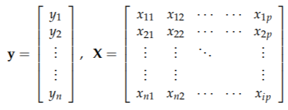
• given Y and X data:
• PCA on X matrix
– define a new variable: principal component (score)
• in multivariate linearity_ Return_ (_MLR_) Some of these new variables are used to model / predict Y
• Y may be univariate or multivariable.
example
#  On data
set.seed(123)

da1 <- marix(c(x1, x2, x3, x4, y), ncol = 5, row = F)
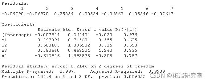
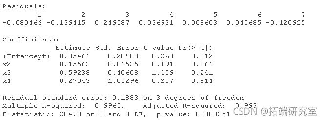
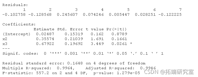
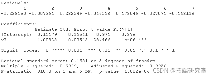
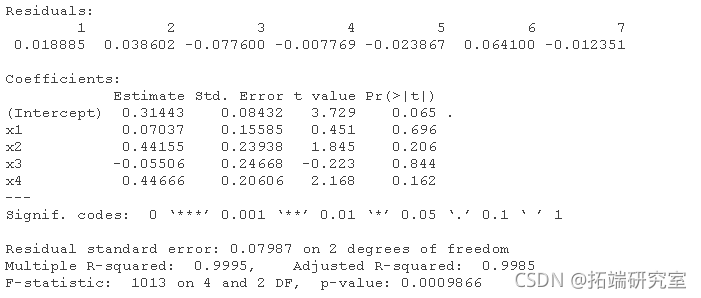
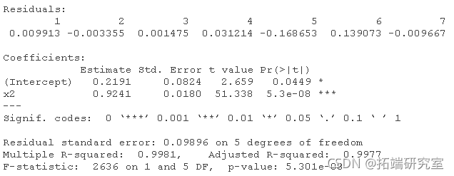
Multiple linear regression and stepwise elimination of variables, manual:
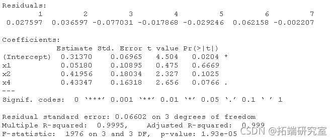
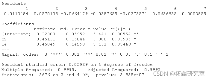
#  For data1: (the correct order will change according to the simulation).
lm(y ~ x1 + x2 + x3 + x4)

lm(y ~ x2 + x3 + x4)


lm(y ~ x2 + x3)


lm(y ~ x3)
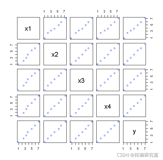
Pairing diagram
pais(atix, ncol = 5, byrow = F
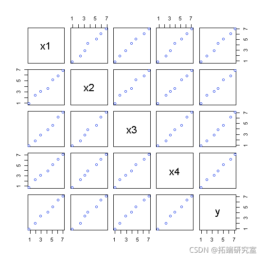
If repeated:
#  For data2:

 lm(y ~ x1 + x2 + x3 + x4)

 lm(y ~ x1 + x2 + x4)


 lm(y ~ x2 + x4)

 lm(y ~ x2)
Plot for dataset 2:
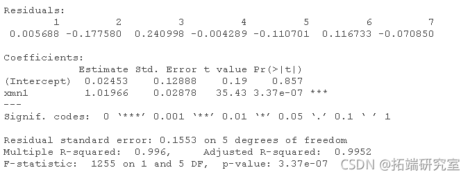
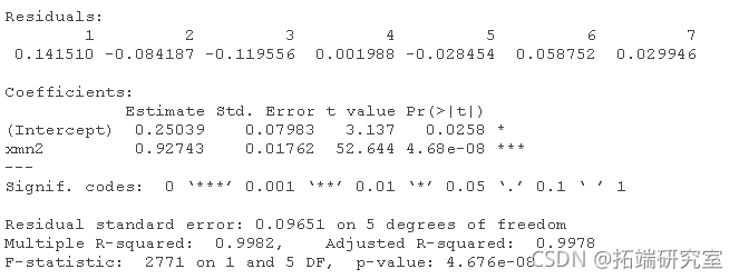
Two data sets were analyzed using the mean of four x's as a single variable:
xn1 <- (dt1\[,1\] + a1\[,2\] + at1\[,3\] + dt1\[,4\])/4
 lm(data1\[,5\] ~ xn1)
 lm(data2\[,5\] ~ xn2)
Check the load of PCA of X data.
#  Almost all variances are explained in the first principal component.
prnmp(dt1\[,1:4\])
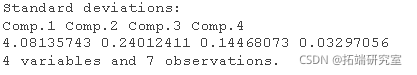
#  Load of the first component
picp(dta1\[,1:4\])$lads\[,1\]

They are almost the same, so that the first principal component is essentially the average of the four variables. Let's save some predicted beta coefficients - a complete set from data 1 and a set from mean analysis:
c1 <- smry(lm(dta1\[,5\] ~ dta1\[,1\] + dta1\[,2\] + ata1\[,3\] +
dt1\[,4\]))$coficns\[,1\]
f <- summry(rm2)$cefets\[,1\]
We now simulate the performance of three methods (complete model, mean (= PCR) and single variable) in 7000 predictions:
#  Simulate the prediction.
error<- 0.2

xn <- (x1 + x2 + x3 + x4)/4
yt2 <- cf\[1\] + cf\[2\] * xn
yht3 <- cf\[1\] + cf\[2\] * x3
bro(c(um((y-hat)^2)/7000 min = "Mean prediction error squared")
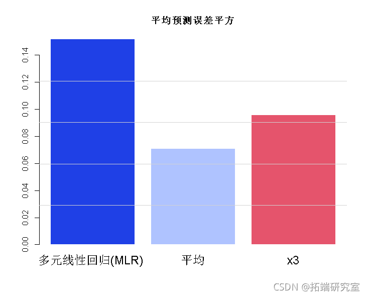
PCR analysis error was the smallest.
Example: spectral type data
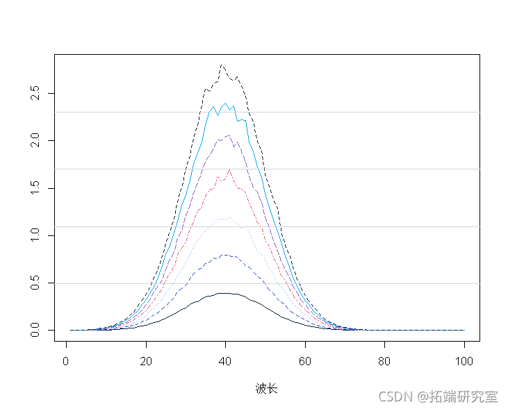
Construct some artificial spectral data: (7 observations, 100 wavelengths)
#  Spectral data example

mapot(t(spcra) )
mtlnes(t(spcra))
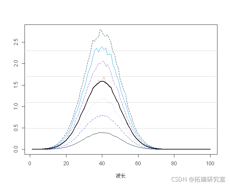
The average spectrum shows that:
mtpot(t(secra))
malies(t(spcta))
mnp <- apply(spcra, 2, mean)
lines(1:100, mnp, lwd = 2)
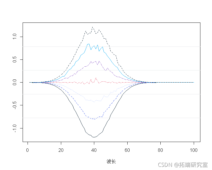
Average central spectrum:
spcamc<-scae(spcta,scale=F)
plot(t(spermc),tpe="")
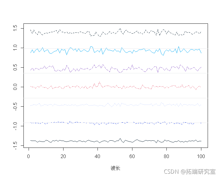
Standardized spectrum:
sptracs<-scale(spetra,scale=T,center=T)
matott(specrams),tye="n",
matlies(t(sectramcs))
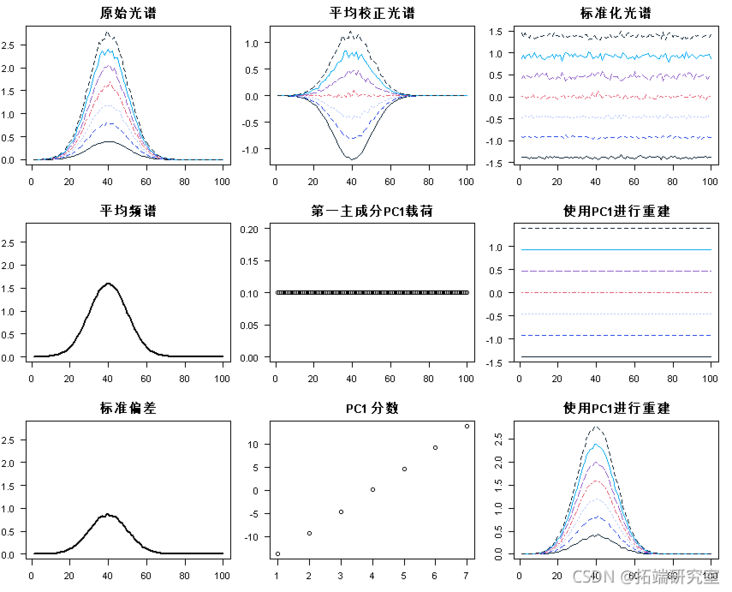
#  PCA of correlation matrix with eigenfunction.
pcaes <- eien(cor(spra))
ladigs <- pces$vectors\[,1\].
score <- peramcs%*%t(t(lodis1))
pred <- soes1 %*% loadings1
##  1-PCA predicted value is converted to original scale and average value.
mtrx(repeasp, 7), nro=7, brw=T)
All graphs collected in a single overview graph:
par(mfrow = c(3, 3)
matlot(t(sectr)
What is PCR?
• data:
• use A principal components t1, t2 Do MLR instead of all (or part) x.
• how many components: determined by cross validation.
How do you do it?
1. Explore data
2. Conduct modeling (select the main component quantity and consider variable selection)
3. Verification (residuals, outliers, effects, etc.)
4. Iterations 2. And 3.
5. Explanation, summary and report.
6. If relevant: predict future values.
Cross validation
• ignore some observations
• fit the model on the remaining (reduced) data
• missing observations from the prediction model: y ˆ i,val
• do this in turn for all observations and calculate the overall model performance:
 (predicted root mean square error)
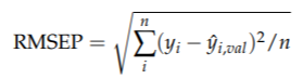
Finally: cross verify all selected components (0, 1, 2,...,...) and draw the model performance
barplot(names.arg)
Select the best score:
• the principal component with the smallest overall error.
Resampling
• cross validation (CV)
• leave on e-_out (LOO)
• Bootstrapping
• a good general approach:
– divide the data into training set and test set.
– use cross validation on training data
– check the performance of the model on the test set
– possible: repeat all of these multiple times (repeat double cross validation)
Cross validation - Principles
• minimize expected forecast errors:
Squared prediction error = Bias2 + variance
• includes "many" PC principal components: low bias, but high variance
• include "few" PC principal components: high bias, but low variance
• choose the best compromise!
Validation - exists at different levels
1. It is divided into three parts: training (50%), verification (25%) and testing (25%)
2. Split into 2: calibration / training (67%) and testing (33%)
CV/bootstrap • is more commonly used in training
3. There is no "fixed segmentation", but repeated segmentation through CV/bootstrap, and then CV in each training group.
4. No segmentation, but use (first level) CV/bootstrap.
5. Fit all data only -- and check for errors.
Example: Car Data
#  Example: using car data.
#  Define the X matrix as a matrix in the data frame.
mtas$X <- as.ix(mcas\[, 2:11\])
#  First, we consider randomly selecting four attributes as the test set
mtcrs_EST<- mtcrs\[tcars$rai == FASE,\] .
tcaTRAIN <- mtars\[tcarstrai == TUE,\] .
Now all the work is carried out on the training data set.
Explore data
We have done this before, so we won't repeat it here
Data modeling
PCR was run with maximum / large number of principal components using pls software package.
#  PCR was run at the maximum / greater fraction using pls software package.
 pls(lomg ~ X , ncop = 10, dta = marsTRAN,
aliaon="LOO")
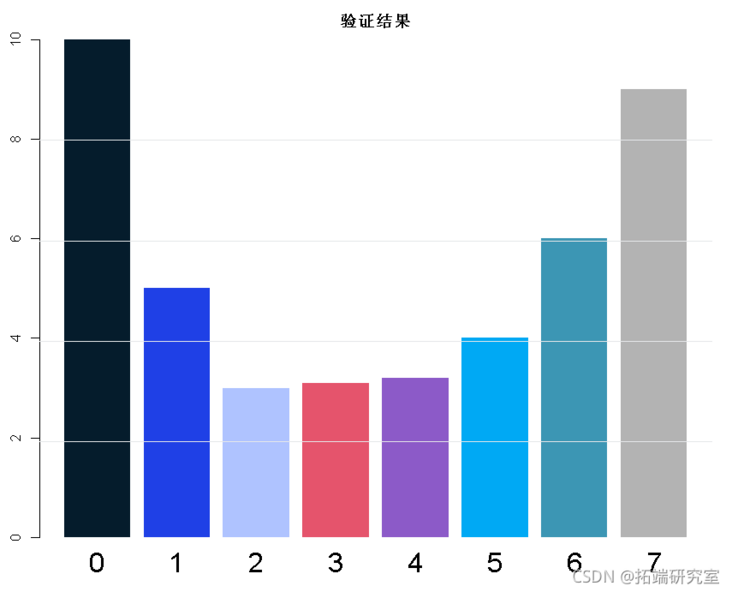
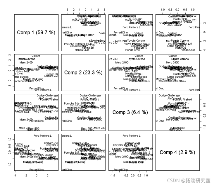
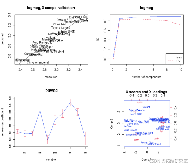
Initial Atlas:
#  Initialized atlas.
par(mfrow = c(2, 2)
plot(mod)
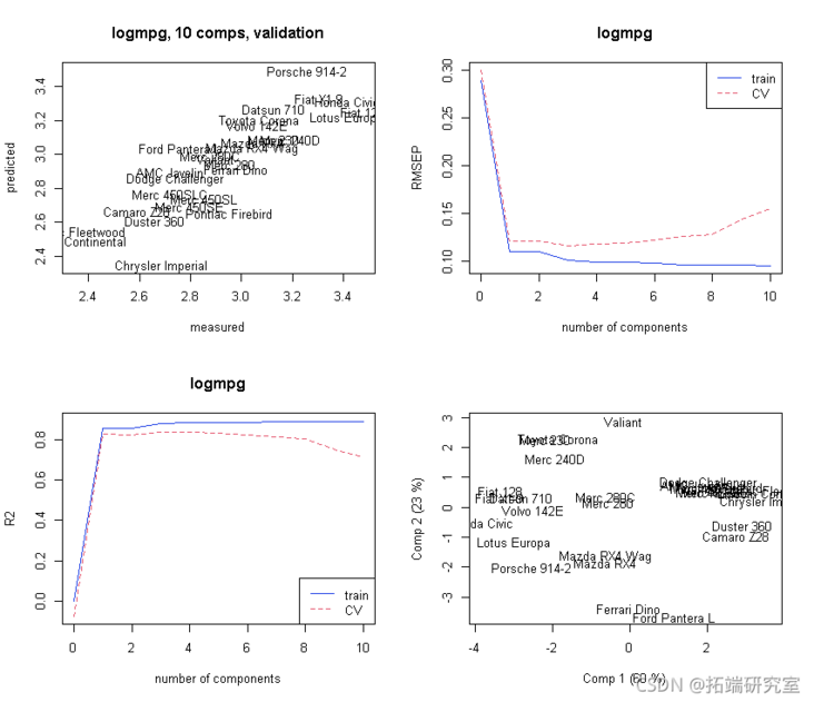
Selection of principal components:
#  Selection of principal components.
#  What happens to segmented CV s.
modseCV <- pcr(lomg ~ X , ncp = 10, dta = marTIN
vai ="CV"
)
#  Initial atlas.
par(mfrow = c(1, 2))
plot(odsC, "vadaion")
Let's look at more principal components:
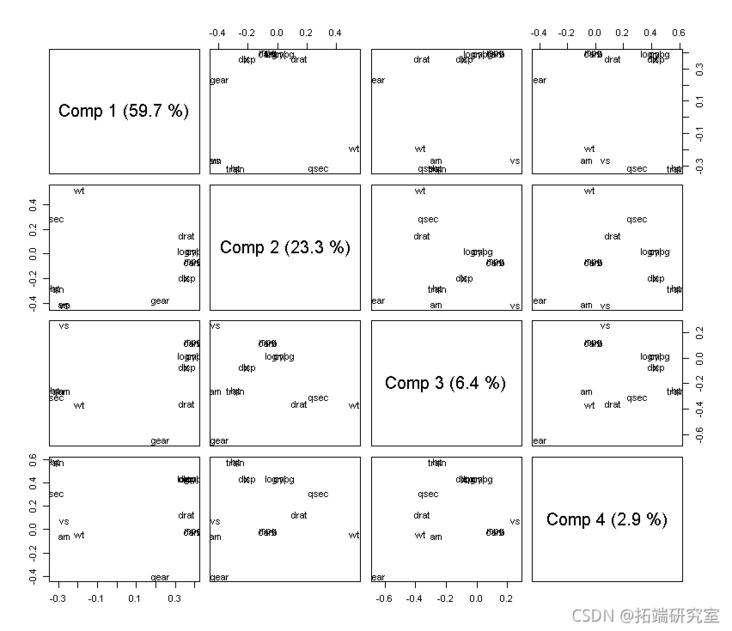
#  Let's look at more principal components.
#  fraction.
scre(mod)
#load
loading(md,cms = 1:4)
We select three principal components:
#  We choose four components
m <-  ncmp = 3, data = mrs_TAI vdon = "LOO", akknie = RUE
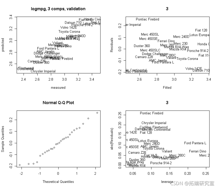
Then: verify:
Let's verify more: use three principal components. We get the predicted residuals from it, so these are (CV) validation versions!
oit <- ppo(mod3, whih = "litin")
plot(obft\[,2\], Rsds)
#  To plot the residual versus the X-lever, we need to find the X-lever.
#  Then find the lever value as the diagonal of the Hat matrix.
#  Based on the fitted X value.
Xf <- sors(md3)
plot(lvge, abs(Rsidals))
text(leage, abs(Reuls))
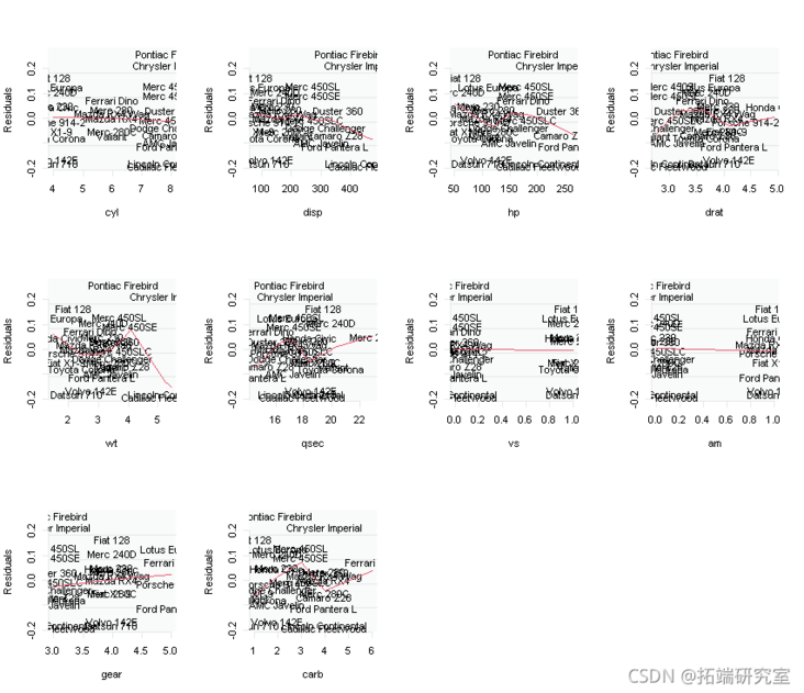
#  Let's also plot the relationship between the residual and each input X.

for ( i in 2:11){
plot(res~masAN\[,i\],type="n")
} 
Explanation / conclusion
Now let's look at the results - "explanation / conclusion":
#  Now let's look at the results  -  4)   "Explanation / conclusion"
par(mfrw = c(2, 2))
#  Plot coefficients with Jacknife uncertainty.
obfi <- red(mod3,, wich = "vltn)
abe(lm(ft\[,2\] ~ fit\[,1\])
plt(mo3, ses = TUE,)
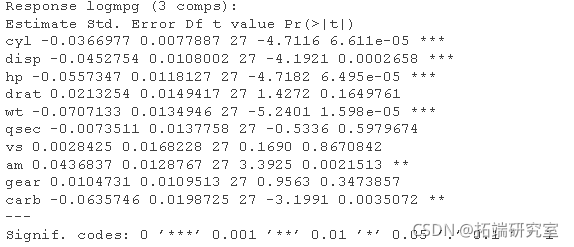
#  Finally, there are some outputs
test(mo3, nm = 3)
forecast
#  Now let's try to predict the four data points in the TEST set.
prdit(md3, nwaa =TEST)
plt(TEST$lgg, pes)
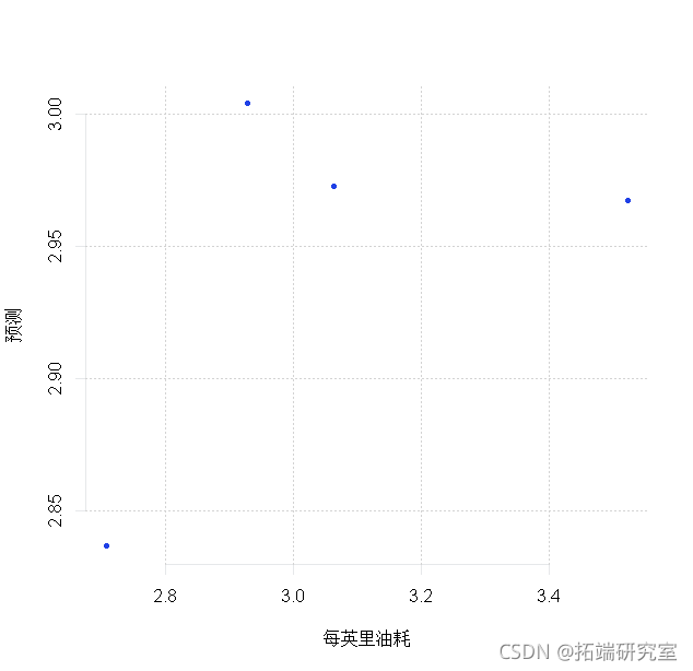
rmsep <- sqrt(men(log - prd)^2))
rmsep