Original link: http://tecdat.cn/?p=24148
Especially in economics / econometrics, modelers do not believe that their models can reflect reality. For example, the yield curve does not follow the three factor Nelson Siegel model, the relationship between stocks and their related factors is not linear, and the volatility does not follow the Garch(1,1) process, or Garch(?,?). We are just trying to find a suitable description of the phenomenon we see.
The development of models is often determined not by our understanding, but by the arrival of new data, which are not suitable for the existing views. Some people can even say that there is no basic model (or data generation process) in reality. As Hansen wrote in the challenge of econometric model selection.
"The model should be regarded as an approximation, which should be taken seriously by econometric theory."
All theories naturally follow the idea of "if this is a process, then we show convergence to real parameters". Convergence is important, but it is a big assumption. Whether there is such a process or such a real model, we don't know what it is. Similarly, especially in the field of Social Sciences, even if there is a real GDP, you can think it is variable.
This discussion leads to the combination of models, or the combination of predicting the future. If we do not know the potential truth, combining different options or different modeling methods may produce better results.
Model average
Let's use three different models to predict time series data. Simple regression (OLS), lifting tree and random forest. Once we have three predictions, we can average them.
#  Load the packages needed to run the code. If you are missing any packages, install them first.

tem <- lappy(c("randomoest", "gb", "quanteg"), librry, charter.oly=T)


#  Regression model.


moelm <- lm(y~x1+x2, data=f)


molrf <- ranmFrst(y~x1+x2, dta=df)

mogm <- gb(ata=df, g.x=1:2, b.y=4
faiy = "gssian", tre.comle = 5, eain.rate = 0.01, bg.fratn = 0.5)


#  Now let's make predictions outside the sample.

#-------------------------------

Tt_ofsamp <- 500


boosf <- pbot(df\_new$x1, df\_new$x2)

rfft <- pf(df\_new$x1, df\_new$x2)

lmt <- pm(df\_new$x1, df\_new$x2)

#  Binding prediction

mtfht <- cbind(bo\_hat, f\_fat, lm_at)

#  Name these columns

c("Boosting", "Random Forest", "OLS")

#  Define a forecast combination scheme.


#  Make room for results.

resls <- st()

#  The first 30 observations serve as the initial window

#  Re estimate the arrival of new observations

it_inw = 30

for(i in 1:leth(A_shes)){
A\_nw$y, mt\_fht,Aeng\_hee= A\_scmes\[i, n_wiow = intwdow )


}

#  This function outputs the MSE of each prediction average scheme.


#  Let's check the MSE of each method.

atr <- apy(ma\_ht, 2, fucon(x) (df\_wy - x)^2 )

apy(ma\_er\[nitnow:Tou\_o_saple, \], 2, fncon(x) 100*( man(x) ) )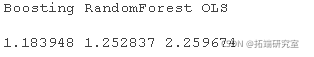
In this case, the most accurate method is to improve. However, in other cases, random forests are better than ascension, depending on the situation. If we use the constrained least squares method, we can obtain almost the most accurate results, but we do not need to select the Boosting and Random Forest methods in advance. Continuing with the introductory discussion, we just don't know which model will provide the best results and when.
Weighted average model fusion prediction
 Is your predictor,
  Time prediction
  , From method
  , and
, and  For example, OLS,
  Lifting tree and
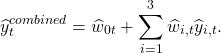
  It's a random forest. You can only take the average value of the forecast:

Usually, this simple average performs very well.
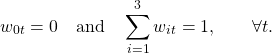
In OLS averaging, we simply project the prediction onto the target, and the resulting coefficient is used as the weight:
This is quite unstable. All predictions have the same goal, so they are likely to be related, which makes it difficult to estimate the coefficients. A good way to the stability factor is to use constrained optimization, that is, you solve the least squares problem, but under the following constraints:
Another method is to average the prediction according to the accuracy of the prediction until it is based on some indicators such as root MSE. We reverse the weights so that more accurate (low RMSE) get more weights.
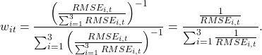
You can draw weights for each method: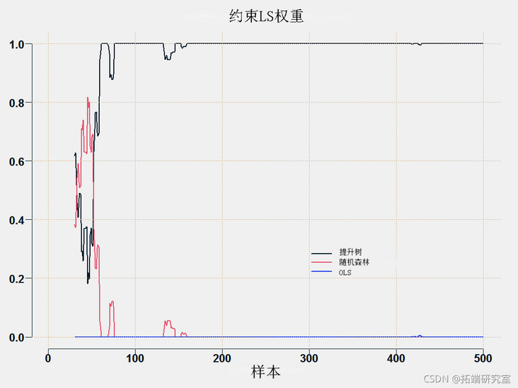
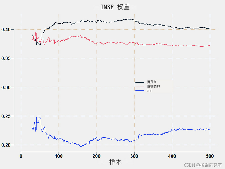
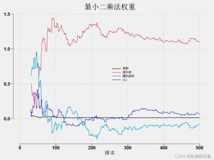
This is the prediction average method.
##  Required subroutines.

er <- funcion(os, red){ man( (os - ped)^2 ) }


##  Different forecast average schemes

##simple


  rd <- aply(a_at, 1, an)

  wehs <- trx( 1/p, now = TT, ncl = p)

  ##  OLS weight


   wgs <- marx( nol=(p+1)T)

for (i in in_wnow:TT) {

  wghs\[i,\] <- lm $oef

pd <- t(eigs\[i,\])%*%c(1, aht\[i,\] )

##  Robust weight


   for (i in iitnow:T) {

    whs\[i,\] <- q(bs\[1:(i-1)\]~ aft\[1:(i-1),\] )$cef

   prd\[i\] <- t(wihs\[i,\] )*c(1, atfha\[i,\])

   ##Variance based on error. Reciprocal of MSE


  for (i in n_no:TT) {

   mp =aply(aerr\[1:(i-1),\]^2,2,ean)/um(aply(mter\[1:(i-1),\]^2,2,man))

  wigs\[i,\] <- (1/tmp)/sum(1/tep)

  ped\[i\] <- t(wits\[i,\] )%*%c(maat\[i,\] )

  ##Using constrained least squares


for (i in itd: wTT) {

  weht\[i,\] <- s1(bs\[1:(i-1)\], a_fat\[1:(i-1),\] )$wigts

  red\[i\] <- t(wehs\[i,\])%*%c(aht\[i,\] )

  ##According to the square function of loss, the best model is selected so far


    tmp <- apy(mt\_fat\[-c(1:iit\_wdow),\], 2, ser, obs= obs\[-c(1:ntwiow)\] )

    for (i in it_idw:TT) {

    wghs\[i,\] <- rp(0,p)

    wihts\[i, min(tep)\] <- 1

    ped\[i\] <- t(wiht\[i,\] )*c(mht\[i,\] )

    } }

MSE <- sr(obs= os\[-c(1: intiow)\], red= red\[-c(1: itwiow)\])
Most popular insights
1.Using lstm and python for time series prediction in Python
2.Using long-term and short-term memory model lstm to predict and analyze time series in python
3.Time series (arima, exponential smoothing) analysis using r language
4.r language multivariate copula GARCH model time series prediction
5.r language copulas and financial time series cases
6.Using r language random fluctuation model sv to deal with random fluctuations in time series
7.tar threshold autoregressive model of r language time series
8.r language k-shape time series clustering method for stock price time series clustering