Series of articles: Learning notes of machine learning practice

Decision tree

• Advantages: the calculation complexity is not high, the output result is easy to understand, is not sensitive to the loss of intermediate value, and can process irrelevant feature data.
• Disadvantages: over matching may occur.
• Applicable data types: discrete and continuous

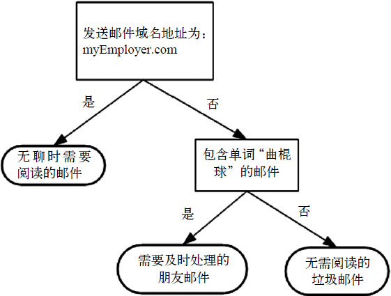
We often use the decision tree to deal with classification problems. Its process is similar to the game of 20 questions: the party participating in the game thinks of something in his mind, and other participants ask him questions. Only 20 questions are allowed to be asked, and the answer to the question can only be right or wrong. People who ask questions gradually narrow the scope of guessing things through inference and decomposition. The flowchart shown in Figure 1 is a decision tree. The rectangle represents the decision block and the ellipse represents the terminating block, indicating that the operation can be terminated after a conclusion has been reached. The left and right arrows from the judgment module are called branch es, which can reach another judgment module or termination module.

Figure 1 constructs an imaginary mail classification system, which first detects the domain name and address of sending mail. If the address is myemployee.com, put it in the category "messages to read when bored". If the email is not from this domain name, check whether the content includes the word hockey. If so, classify the email as "friend email that needs to be handled in time", otherwise classify the email as "spam that does not need to be read".

The k-nearest neighbor algorithm introduced in Chapter 2 can complete many classification tasks, but its biggest disadvantage is that it can not give the internal meaning of data. The main advantage of decision tree is that the data form is very easy to understand.

The decision tree algorithm constructed in this chapter can read the data set and build a decision tree similar to figure 1. Decision tree can extract a series of rules from the data set. The process of rule creation is the process of machine learning. Now that we have a general understanding of what the decision tree can do, we will learn how to construct a decision tree from a pile of raw data. Firstly, we discuss the method of constructing the decision tree and how to write the Python code of constructing the tree; Then, some methods to measure the success rate of the algorithm are proposed; Finally, the classifier is established by recursion.

1, Construction of decision tree

When constructing the decision tree, the first problem we need to solve is which feature on the current data set plays a decisive role in data classification. In order to find the decisive features and divide the best results, we must evaluate each feature. Assuming that the feature to be divided has been selected according to a certain method, the original data set will be divided into several data subsets according to this feature. This data subset is distributed on all branches of the decision point (key feature). If the data under a branch belongs to the same type, there is no need to further divide the data set. If the data in the data subset does not belong to the same type, the process of dividing the data subset needs to be repeated recursively until the data type in each data subset is the same.

The process of creating a branch is represented by pseudo code as follows:

Check whether each sub item in the dataset belongs to the same type:
　　If yes, the type label is returned
　　Otherwise:
　　　　Find the best features to divide the dataset
　　　　Partition dataset
　　　　Create branch node
　　　　For each data subset divided:
　　　　　　Call this algorithm recursively and add the returned result to the branch node
　　　　Return branch node

Note: pseudo code is a recursive function.

General process of decision tree:

1. Collect data: any method can be used.
2. Prepare data: the tree construction algorithm is only applicable to nominal data, so numerical data must be discretized.
3. Analyze data: any method can be used. After constructing the tree, we should check whether the graph meets the expectations.
4. Training algorithm: construct the data structure of the tree.
5. Test algorithm: use the experience tree to calculate the error rate.
6. Using algorithm: this step can be applied to any supervised learning algorithm, and using decision tree can better understand the internal meaning of data.

Some decision tree algorithms use dichotomy to divide data, which is not used in this book. If the data is divided according to a certain attribute, four possible values will be generated. We will divide the data into four blocks and create four different branches.

This book will use ID3 algorithm to divide data sets. This algorithm deals with how to divide data sets and when to stop dividing data sets (for further information, see http://en.wikipedia.org/wiki/ID3_algorithm ). Each time we divide the dataset, we only select one feature attribute, so which feature should be selected as the reference attribute of the division?

The data in Table 1 contains five marine animals, including whether they can survive without coming out of the water and whether they have feet poof. We can divide these animals into two categories: fish and non fish.

Table 1 marine biological data

	Can we survive without coming to the surface	Are there fins	Belonging to fish
1	yes	yes	yes
2	yes	yes	yes
3	yes	no	no
4	no	yes	no
5	no	yes	no

1.1 information gain

The general principle of dividing data sets is to make disordered data more orderly. We can use many methods to partition data sets, but each method has its own advantages and disadvantages. One way to organize disordered data is to use information theory to measure information. Information theory is a branch of science that quantifies and processes information. We can use information theory to quantify the content of quantitative information before or after dividing the data.

Before and after dividing the data set, the change of information becomes information gain. We can calculate the information gain obtained by dividing the data set for each feature. The feature with the highest information gain is the best choice.

For something
The greater the uncertainty, the greater the entropy, and the greater the amount of information needed to determine the matter;
The smaller the uncertainty, the smaller the entropy, and the smaller the amount of information required to determine the matter.

(personal understanding: changing the disordered data into ordered data before and after is information gain, and the degree of confusion of data information is called entropy).

The measurement of set information is called Shannon entropy or entropy for short.

Entropy is defined as the expected value of information. We first determine the definition of information:

If the transaction to be classified may be divided into multiple classifications, the symbol \ (x_i \) is defined as:

Where \ (p(x_i) \) is the probability of selecting the classification.

In order to calculate entropy, we need to calculate the expected value of information contained in all types of possible values, which is obtained by the following formula:

Where \ (n \) is the number of classifications.

The Python function for calculating information entropy is given below. Create a file named trees.py and add the following code:

from math import log

# H(x) = -\sum_{i = 1}^nP(X_i)log_2P(X_i)
def calsShannonEnt(dataSet):
    numEntries = len(dataSet)
    labelCounts = {}
    
    # Create a dictionary for all possible words
    for dataVec in dataSet:
        label = dataVec[-1]
        if label not in labelCounts.keys(): # Create a dictionary for all possible classifications
            labelCounts[label] = 0
        labelCounts[label] += 1
    
    shannonEnt = 0.0
    for key in labelCounts.keys():
        prob = float(labelCounts[key]) / numEntries
        shannonEnt -= prob * log(prob, 2) # Find logarithm based on 2
    return shannonEnt

Code Description:

• First, calculate the total number of instances in the dataset. We can calculate this value when necessary, but since this value is used many times in the code, in order to improve code efficiency, we explicitly declare a variable to save the total number of instances.
• Then, create a data dictionary whose key value is the value of the last column. If the current key value does not exist, expand the dictionary and add the current key value to the dictionary. Each key value records the coarseness of the current category.
• Finally, the occurrence frequency of all class labels is used to calculate the probability of class occurrence. We will use this probability to calculate Shannon entropy and count the times of all class labels.

In the trees.py file, we use the createDateSet() function to get some sample data:

def creatDataSet():
    dataSet = [
        [1, 1, 'yes'],
        [1, 1, 'yes'],
        [1, 0, 'no'],
        [0, 1, 'no'],
        [0, 1, 'no'],
    ]
    labels = ['no surfacng', 'flippers']
    return dataSet, labels

The higher the entropy, the more mixed data. After obtaining the entropy, we can divide the data set according to the method of obtaining the maximum information gain.

Another method to measure the disorder degree of a set is Gini impurity, which is simply to randomly select sub items from a data set to measure the probability that they are misclassified into other groups.

1.2 dividing data sets

We will calculate the information entropy of the result of dividing the data set according to each feature, and then judge which feature is the best way to divide the data mart.

Add code to divide the dataset:

def splitDataSet(dataSet, axis, value):
    retDataSet = []  # Create a new list object
    for featVec in dataSet:
        if featVec[axis] == value:
            reducedFeatVec = featVec[:axis]
            reducedFeatVec.extend(featVec[axis + 1:])
            retDataSet.append(reducedFeatVec)  # extract
    return retDataSet

The function uses three input parameters: dataset with partition, characteristics of the partition dataset, and the value of the characteristics to be returned. The function first selects the data with the axis feature value in the data set, removes the axis feature from this part of the data, and returns.

Test this function and the effect is as follows:

>>> import trees
>>> myDat, labels = trees.createDataSet()
>>> myDat
[[1, 1, 'yes'], [1, 1, 'yes'], [1, 0, 'no'], [0, 1, 'no'], [0, 1, 'no']]
>>> trees.splitDataSet(myDat,0,1)
[[1, 'yes'], [1, 'yes'], [0, 'no']]
>>> trees.splitDataSet(myDat,0,0) 
[[1, 'no'], [1, 'no']]

Next, we will traverse the entire data set and cycle through Shannon entropy and splitDataSet() function to find the best feature division method.

def chooseBestFeatureToSplit(dataSet):
    numFeatures = len(dataSet[0]) - 1
    baseEntropy = calsShannonEnt(dataSet)
    bestInfoGain = 0.0
    bestFeature = -1
    for i in range(numFeatures):
        featList = [example[i] for example in dataSet]
        uniqueVals = set(featList)
        newEntropy = 0.0
        for value in uniqueVals:
            subDataSet = splitDataSet(dataSet, i, value)
            prob = len(subDataSet) / float(len(dataSet))
            newEntropy += prob * calsShannonEnt(subDataSet)
        infoGain = baseEntropy - newEntropy
        if infoGain > bestInfoGain:
            bestInfoGain = infoGain
            bestFeature = i
    return bestFeature

Function selects the first feature for partition.

1.3 recursive construction of decision tree

The sub functional modules required to construct the decision tree have been introduced. The algorithm flow of constructing the decision tree is as follows:

1. Get the original data set,
2. The dataset is divided based on the best attribute value. Since there may be more than two eigenvalues, there may be dataset division greater than two branches.
3. After the first partition, the data will be passed down to the next node of the tree branch. On this node, we can partition the data again. We can use the principle of recursion to deal with data sets.
4. The condition for the end of recursion is that the program traverses all the attributes that divide the data set, or all instances under each branch have the same classification.

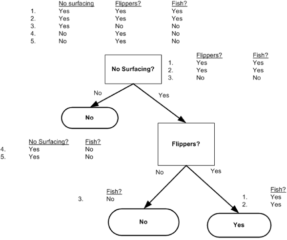
See Figure 2:

Add the following program code in trees.py:

import operator

def majority(classList):
    classCount = {}
    for vote in classList:
        if vote not in classCount.key(): classCount[vote] = 0
        classCount[vote] += 1
    sortedclassCount = sorted(classCount.iteritems(),
                              key=operator.itemgetter(1),
                              reverse=True)
    return sortedclassCount[0][0]

# Create tree
def createTree(dataSet, labels):
    classList = [example[-1] for example in dataSet]
    # If the type is exactly the same, continue the division
    if classList.count(classList[0]) == len(classList):
        return classList[0]
    # When all the features are traversed, the feature with the most occurrences is returned
    if len(dataSet[0]) == 1:
        return majority(classList)
    bestFeat = chooseBestFeatureToSplit(dataSet=dataSet)
    bestFeatLabel = labels[bestFeat]
    myTree = {bestFeatLabel: {}}
    del (labels[bestFeat])
    # Get all attribute values contained in the list
    featValues = [example[bestFeat] for example in dataSet]
    uniqueVals = set(featValues)
    for value in uniqueVals:
        sublabels = labels[:]  # Copy labels list
        myTree[bestFeatLabel][value] = createTree(
            splitDataSet(dataSet, bestFeat, value), sublabels)  # Recursive construction of subtree
    return myTree

The majorityCnt function counts the frequency of each type label in the classList list and returns the category name with the most occurrences.

The createTree function uses two input parameters: dataSet dataset and label list labels

The tag list contains the tags of all features in the dataset. The algorithm itself does not need this variable, but in order to give a clear meaning of the data, we provide it as an input parameter.

The above code first creates a list variable named classList, which contains all the class labels of the dataset. The list variable classList contains all the class labels of the dataset. If the first stop condition of a recursive function is that all class labels are exactly the same, the class label is returned directly. The second stop condition for recursive functions is that after using all the features, the dataset cannot be divided into groups containing only unique categories. Here, the majorityCnt function is used to select the category with the most occurrences as the return value.

Next, the program starts to create the tree. Here, the Python dictionary type is directly used to store the tree information. The dictionary variable myTree stores all the information of the tree. The best feature selected from the current dataset is stored in the variable bestFeat to obtain all attribute values contained in the list.

Finally, the code traverses all the attribute values contained in the currently selected feature, recurses the standby function createTree() on each dataset partition, and the return value obtained will be inserted into the dictionary variable myTree. Therefore, when the function terminates execution, many dictionary data representing leaf node information will be nested in the dictionary.

Note that subLabels = labels [:] copies the class label because the value of the label list will be changed in a recursive call to the createTree function.

Test these functions:

>>> import trees
>>> myDat, labels = trees.createDataSet()
>>> myTree = trees.createTree(myDat,labels) 
>>> myTree
{'no surfacng': {0: 'no', 1: {'flippers': {0: 'no', 1: 'yes'}}}}

2, Draw a tree using the Matplotlib annotation

In the previous section, we learned how to create a tree from a dataset. However, the representation of the dictionary is very difficult to understand, and it is difficult to draw graphics directly. In this section, we will create a tree diagram using the Matplotlib library. The main advantage of decision tree is that it is intuitive and easy to understand. If it can't be displayed intuitively, it can't give full play to its advantages. Although the graphics library we used in the previous chapters is very powerful, Python does not provide a tool for drawing trees, so we must draw tree graphs ourselves. In this section, we will learn how to write code to draw the decision tree shown in Figure 3.

2.1 Matplotlib annotation

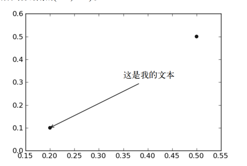
Matplotlib provides an annotation tool, annotations, which is very useful. It can add text annotations to data graphics. Annotations are often used to interpret the contents of data. Because the text description directly above the data is very ugly, the tool embedded supports the scribing tool with arrow, so that we can point to the data location in other appropriate places, add description information here and explain the data content. As shown in Figure 4, there is a point at the position of the coordinate \ ((0.2, 0.1) \), we put the description information of the point at the position of \ ((0.35, 0.3) \), and point to the data point \ ((0.2, 0.1) \) with an arrow.

Using the annotation function of Matplotlib to draw a tree diagram, it can color the text and provide a variety of shapes for selection, and we can also reverse the arrow and point it to the text box instead of the data point. Open a text editor, create a new file named treePlotter.py, and enter the following program code.

import matplotlib.pyplot as plt

# Define text box and arrow formats
decisionNode = dict(boxstyle="sawtooth", fc="0.8")
leafNode = dict(boxstyle="round4", fc="0.8")
arrow_args = dict(arrowstyle="<-")


# Draw annotation with arrow
def plotNode(nodeTxt, centerPt, parentPt, nodeType):
    createPlot.axl.annotate(nodeTxt,
                            xy=parentPt,
                            xycoords='axes fraction',
                            xytext=centerPt,
                            textcoords='axes fraction',
                            va="center",
                            ha="center",
                            bbox=nodeType,
                            arrowprops=arrow_args)

# createPlot version 1
def createPlot():
    fig = plt.figure(1, facecolor='white')
    fig.clf()  # Empty drawing area
    createPlot.axl = plt.subplot(111, frameon=False)
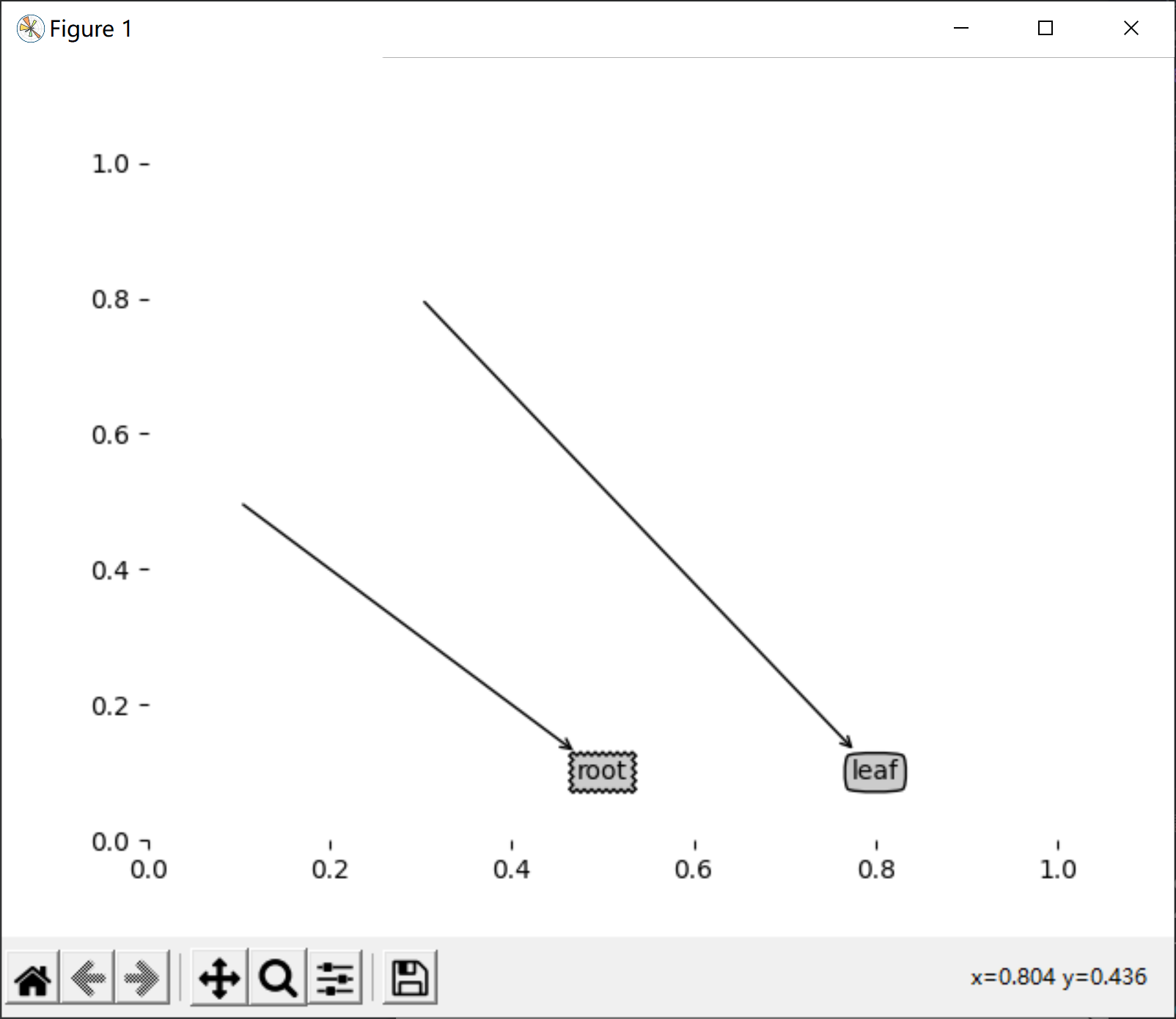
    plotNode(U'Decision node', (0.5, 0.1), (0.1, 0.5), decisionNode)
    plotNode(U'Leaf node', (0.8, 0.1), (0.3, 0.8), leafNode)
    plt.show()


createPlot()

Based on this example, now learn to draw the whole tree.

2.2 construct annotation tree

Drawing a complete tree requires some skills. Although we have \ (x,y \) coordinates, how to place all tree nodes is a problem. We must know how many leaf nodes there are so that we can correctly determine the length of the \ (x \) axis; We also need to know how many layers the tree has so that we can correctly determine the height of the \ (Y \) axis. Here, we define two new functions getNumLeafs() and getTreeDepth() to obtain the number of leaf nodes and the number of layers of the tree. See the following program and add these two functions to the file treePlotter.py.

This code is different from the original book because the Python version is different. Mainly in the following two aspects:

1. 1. The creation of firststr is different: for specific questions, please click: (firstStr creation problem)
2. if judgment statements are different: for specific questions, click: (if judgment statements are different)

# Get the number of leaf nodes
def getNumLeafs(myTree):
    numLeafs = 0
    firstSides = list(myTree.keys())
    firstStr = firstSides[0]  # Find the first element of the input
    secondDict = myTree[firstStr]
    for key in secondDict.keys():
        if type(secondDict[key]) == dict:
            numLeafs += getNumLeafs(secondDict[key])
        else:
            numLeafs += 1
    return numLeafs


# Gets the number of layers of the tree
def getTreeDepth(myTree):
    maxDepth = 0
    firstSides = list(myTree.keys())
    firstStr = firstSides[0]  # Find the first element of the input
    secondDict = myTree[firstStr]
    for key in secondDict.keys():
        if type(secondDict[key]) == dict:
            thisDepth = 1 + getTreeDepth(secondDict[key])
        else:
            thisDepth = 1
        if thisDepth > maxDepth:
            maxDepth = thisDepth
    return maxDepth

The two functions in the above program have the same structure, and we will use them later.

The data structure used here shows how to store tree information in Python dictionary types. The first keyword is the category label that divides the dataset for the first time, and the attached value represents the value of the child node. Starting from the first keyword, we can traverse all child nodes of the whole tree. Use the type() function provided by Python to determine whether the child node is a dictionary type. If the child node is of dictionary type, it is also a judgment node, and the getnumleafs () function needs to be called recursively. The getNumLeafs() function traverses the whole tree, accumulates the number of leaf nodes, and returns the value. The second function getTreeDepth() calculates the number of judgment nodes encountered during traversal. The termination condition of this function is the leaf node. Once the leaf node is reached, it will be returned from the recursive call, and the variable for calculating the tree depth will be added by one. In order to save everyone's time, the function retrieveTree outputs the pre stored tree information, avoiding the trouble of creating a tree from the data every time you test the code. Add the following code to the file treePlotter.py:

#Output the pre stored tree information to avoid the trouble of creating a tree from the data every time the test code
def retrieveTree(i):
    listOfTrees = [{'no surfacing':{0:'no',1:{'flippers':{0:'no',1:'yes'}}}},
                   {'no surfacing':{0:'no',1:{'flippers':{0:{'head':{0:'no',1:'yes'}},1:'no'}}}}
                   ]
    return listOfTrees[i]

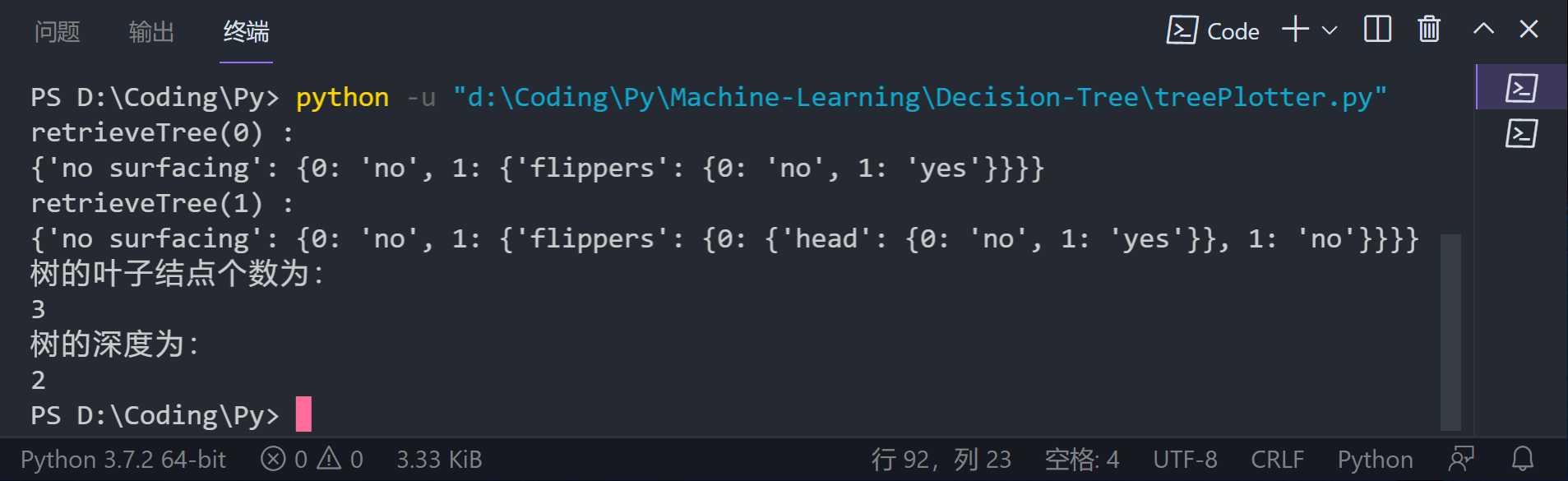
print('retrieveTree(0) : \n{}'.format(retrieveTree(0)))
print('retrieveTree(1) : \n{}'.format(retrieveTree(1)))

myTree = retrieveTree(0)
print('The number of leaf nodes of the tree is:\n{}'.format(getNumLeafs(myTree)))
print('The depth of the tree is: \n{}'.format(getTreeDepth(myTree)))

2.3. Construct annotation tree

#Fill in text information between parent and child nodes
def plotMidText(cntrPt, parentPt, txtString):
    xMid = (parentPt[0] - cntrPt[0]) / 2.0 + cntrPt[0]
    yMid = (parentPt[1] - cntrPt[1]) / 2.0 + cntrPt[1]
    createPlot.axl.text(xMid, yMid, txtString)


#Draw a tree
def plotTree(myTree, parentPt, nodeTxt):
    numLeafs = getNumLeafs(myTree)  #Calculate the width of the tree
    depth = getTreeDepth(myTree)  #Calculate the height of the tree
    firstStr = list(myTree.keys())[0]
    plotTree.totalW = float(getNumLeafs(myTree))  #Width of the storage tree
    plotTree.totalD = float(getTreeDepth(myTree))  #Depth of the storage tree
    cntrPt = (plotTree.xOff + (1.0 + float(numLeafs)) / 2.0 / plotTree.totalW,
              plotTree.yOff)
    #cntrPt = (plotTree.xOff + (0.5/plotTree.totalW + float(numLeafs))/2.0/plotTree.totalW,plotTree.yOff)
    plotMidText(cntrPt, parentPt, nodeTxt)  #Tag child node attribute values
    plotNode(firstStr, cntrPt, parentPt, decisionNode)
    secondDict = myTree[firstStr]
    plotTree.yOff = plotTree.yOff - 1.0 / plotTree.totalD
    for key in secondDict.keys():
        if type(secondDict[key]) == dict:
            plotTree(secondDict[key], cntrPt, str(key))
        else:
            plotTree.xOff = plotTree.xOff + 1.0 / plotTree.totalW
            plotNode(secondDict[key], (plotTree.xOff, plotTree.yOff), cntrPt,
                     leafNode)
            plotMidText((plotTree.xOff, plotTree.yOff), cntrPt, str(key))
    plotTree.yOff = plotTree.yOff + 1.0 / plotTree.totalD


#createPlot version 2
def createPlot(inTree):
    fig = plt.figure(1, facecolor='white')
    fig.clf()
    axpropps = dict(xticks=[], yticks=[])
    createPlot.axl = plt.subplot(111, frameon=False, **axpropps)
    plotTree.totalW = float(getNumLeafs(inTree))  #Width of the storage tree
    plotTree.totalD = float(getTreeDepth(inTree))  #Depth of the storage tree
    plotTree.xOff = -0.5 / plotTree.totalW  #xOff and yOff track the position of the drawn node and the appropriate position of the next node.
    plotTree.yOff = 1.0
    plotTree(inTree, (0.5, 1.0), '')
    plt.show()


myTree = retrieveTree(0)
createPlot(myTree)

Note: during the execution, I found that the image could not be fully displayed, so I clicked the setting to adjust the size and position of the image, as shown in the figure below.

2.4. Change dictionary

#Fill in text information between parent and child nodes
def plotMidText(cntrPt,parentPt,txtString):
    xMid = (parentPt[0] - cntrPt[0])/2.0 + cntrPt[0]
    yMid = (parentPt[1] - cntrPt[1])/2.0 + cntrPt[1]
    createPlot.axl.text(xMid,yMid,txtString)
 
#Draw a tree
def plotTree(myTree,parentPt,nodeTxt):
    numLeafs = getNumLeafs(myTree) #Calculate the width of the tree
    depth = getTreeDepth(myTree) #Calculate the height of the tree
    firstStr = list(myTree.keys())[0]
    plotTree.totalW = float(getNumLeafs(myTree))  #Width of the storage tree
    plotTree.totalD = float(getTreeDepth(myTree)) #Depth of the storage tree
    cntrPt = (plotTree.xOff + (1.0 + float(numLeafs))/2.0/plotTree.totalW,plotTree.yOff)
    #cntrPt = (plotTree.xOff + (0.5/plotTree.totalW + float(numLeafs))/2.0/plotTree.totalW,plotTree.yOff)
    plotMidText(cntrPt,parentPt,nodeTxt) #Tag child node attribute values
    plotNode(firstStr,cntrPt,parentPt,decisionNode)
    secondDict = myTree[firstStr]
    plotTree.yOff = plotTree.yOff - 1.0/plotTree.totalD
    for key in secondDict.keys():
        if type(secondDict[key]) == dict:
            plotTree(secondDict[key],cntrPt,str(key))
        else:
            plotTree.xOff = plotTree.xOff + 1.0/plotTree.totalW
            plotNode(secondDict[key],(plotTree.xOff,plotTree.yOff),cntrPt,leafNode)
            plotMidText((plotTree.xOff,plotTree.yOff),cntrPt,str(key))
    plotTree.yOff = plotTree.yOff + 1.0/plotTree.totalD
 
#createPlot version 2
def createPlot(inTree):
    fig = plt.figure(1,facecolor='white')
    fig.clf()
    axpropps = dict(xticks = [],yticks = [])
    createPlot.axl = plt.subplot(111, frameon = False, **axpropps)
    plotTree.totalW = float(getNumLeafs(inTree))  #Width of the storage tree
    plotTree.totalD = float(getTreeDepth(inTree)) #Depth of the storage tree
    plotTree.xOff = -0.5/plotTree.totalW  #xOff and yOff track the position of the drawn node and the appropriate position of the next node.
    plotTree.yOff = 1.0
    plotTree(inTree,(0.5,1.0),'')
    plt.show()

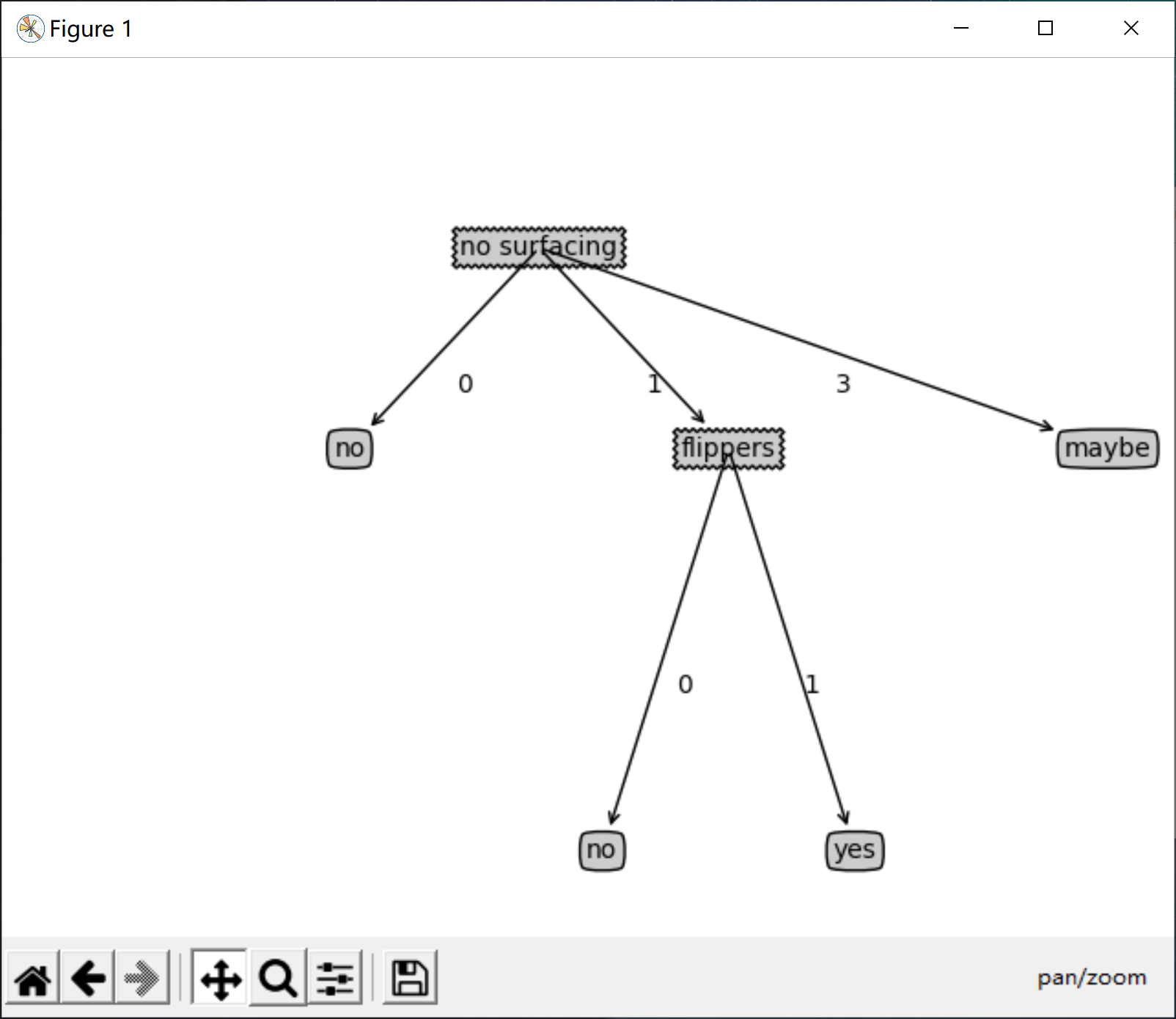
myTree = retrieveTree(0)
myTree['no surfacing'][3] = 'maybe'
print('myTree : \n{}'.format(myTree))
createPlot(myTree)

The operation results are as follows

myTree : 
{'no surfacing': {0: 'no', 1: {'flippers': {0: 'no', 1: 'yes'}}, 3: 'maybe'}}

3, Test and store classifiers

3.1 test algorithm: use decision tree for classification

After constructing the decision tree based on the training data, we can use it to classify the actual data. When performing data classification, you need a decision tree and a label vector for the decision tree. Then, the program compares the test data with the values on the decision tree, and recursively executes the process until it enters the leaf node; Finally, the test data is defined as the type of leaf node.

Functions using decision tree classification: