Today, let's learn more about Vision Transformer. timm based code.
1. Patch Embedding
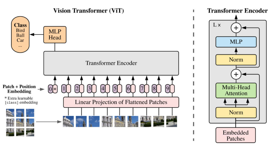
Transformer was originally used to do NLP work, so ViT's primary task is to convert the graph into word structure. The method adopted here is to divide the picture into small blocks, as shown in the lower left corner of the above figure. Each small block is equivalent to a word in the sentence. Here, each Patch is called a Patch, and Patch Embedding is to compress each Patch into a vector of a certain dimension through a fully connected network.
Here is the part about Patch Embedding in the VisionTransformer source code:
# Default img_size=224, patch_size=16,in_chans=3,embed_dim=768,
self.patch_embed = embed_layer(
    img_size=img_size, patch_size=patch_size,
    in_chans=in_chans, embed_dim=embed_dim)
And embedded_ Layer is actually PatchEmbed:
class PatchEmbed(nn.Module):
    """ 2D Image to Patch Embedding
    """
    def __init__(self, img_size=224, patch_size=16, in_chans=3, embed_dim=768, norm_layer=None, flatten=True):
        super().__init__()
        # img_size = (img_size, img_size)
        img_size = to_2tuple(img_size)
        patch_size = to_2tuple(patch_size)
        self.img_size = img_size
        self.patch_size = patch_size
        self.grid_size = (img_size[0] // patch_size[0], img_size[1] // patch_size[1])
        self.num_patches = self.grid_size[0] * self.grid_size[1]
        self.flatten = flatten
        #  Input channel, output channel, convolution kernel size, step size
        # C*H*W->embed_dim*grid_size*grid_size
        self.proj = nn.Conv2d(in_chans, embed_dim, kernel_size=patch_size, stride=patch_size)
        self.norm = norm_layer(embed_dim) if norm_layer else nn.Identity()

    def forward(self, x):
        B, C, H, W = x.shape
        assert H == self.img_size[0] and W == self.img_size[1], \
            f"Input image size ({H}*{W}) doesn't match model ({self.img_size[0]}*{self.img_size[1]})."
        x = self.proj(x)
        if self.flatten:
            x = x.flatten(2).transpose(1, 2)  # BCHW -> BNC
        x = self.norm(x)
        return x
Although proj uses convolution, it actually connects each patch to the same fully connected network and converts each patch into a vector. The dimension of x is (B, C, H, w), where B is batch size, C is usually three channels, H and W are the height and width of the picture respectively, while the output is (B, N, e), B is still batch size, n is the number of patches after each graph is cut into patches, and E is embedded_ Size, each patch will be converted into a vector through a fully connected network. E is the length of this vector. According to the principle of convolution, it can also be understood as the number of features of each patch.
2. Positional Encoding
The image is divided into patches, and then each patch is converted into embedding. The next step is to add location information to embedding. The methods of generating location information are mainly divided into two categories: one is directly generated by fixed algorithm, and the other is obtained by training. However, the way of adding location information is relatively unified and rough.
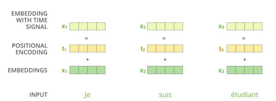
Generate a position vector whose length is consistent with patch embedding, and then add it directly. So what does this position vector look like?

For example, if the length of patch embedding is 4, the length of position vector is also 4, and each position has a value in [- 1,1].
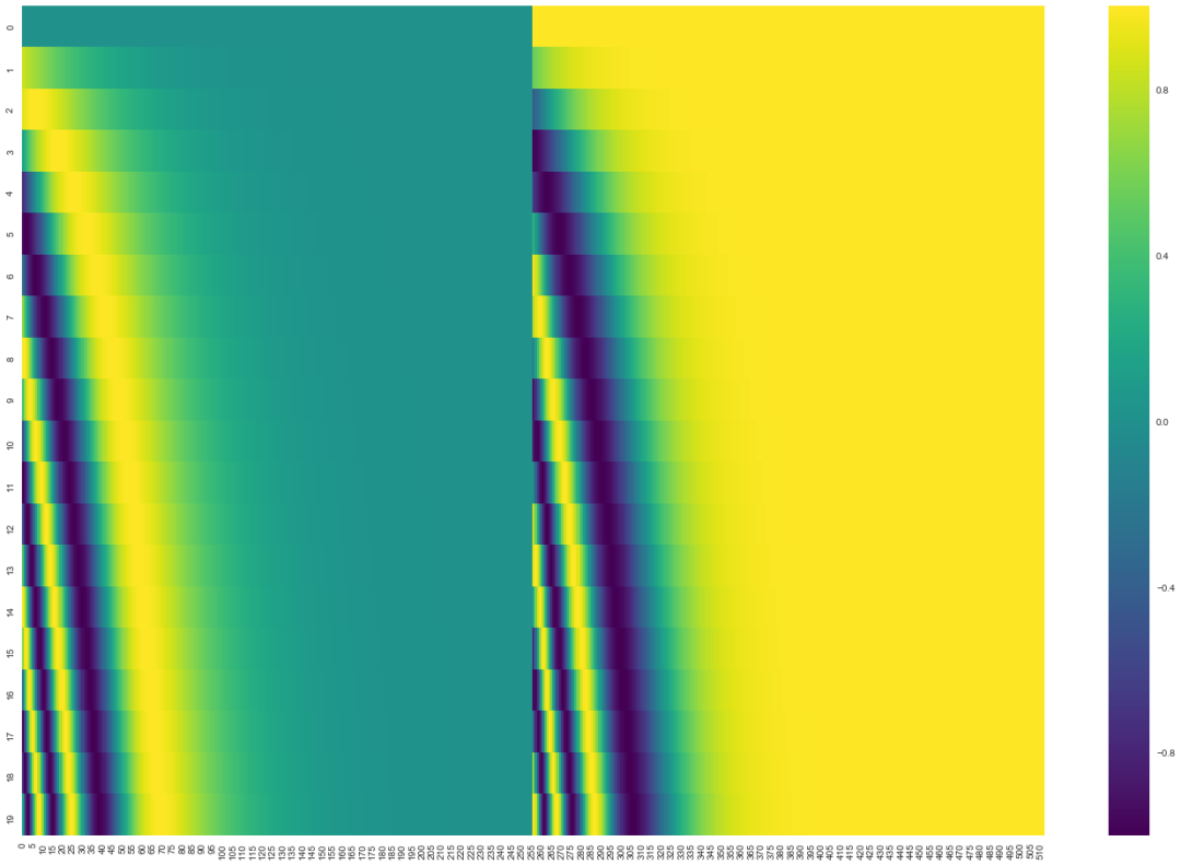
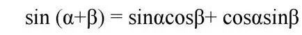
Suppose you cut a graph into 20 patch es and the embedding length is 512, then the position vector can be the above (get_timing_signal_1d function in tensor2tensor). Each line represents a position vector. The first line is the position vector of position 0 and the second line is the position vector of position 1.
The position vector can also be as follows (refer to [1], [4]):
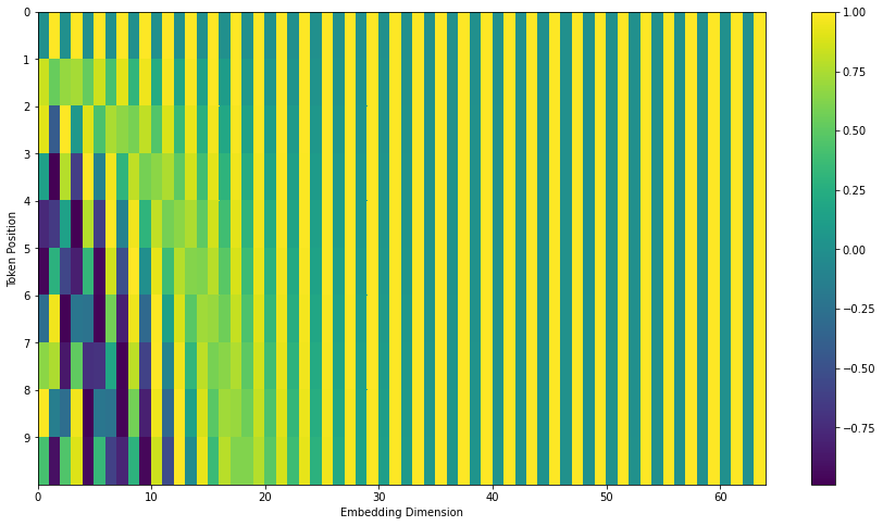
The formula is as follows:
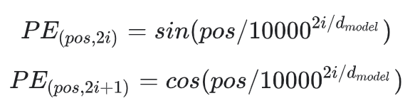
pos is the position of the word in the sentence or the position of the patch in the figure, while i corresponds to the position of embedding, and dmodel corresponds to the length of patch embedding,. Here's why we need to add this location code and what effect it will have in the future. When we observe the last two pictures, we can find that the location code changes with the location. The greater the location difference, the greater the vector difference. In the NLP course, it is said that converting a word into a vector is like mapping a word to the position of a high-dimensional space. Words with similar meanings will be closer in the high-dimensional space. Adding a position vector will make words with similar positions closer and words with far positions farther away. Then, why use cos and sin? The author's explanation is that the relative position between words can be obtained by using sin and cos coding.

Here I understand that according to these two formulas, when we know sin(pos+k), cos(pos+k), and then sin(pos) and cos(pos), we can calculate the value of K, and we can calculate it by addition, subtraction, multiplication and division. Therefore, this coding method can not only express the position of words, but also express the relative position between words.
Let's look at the implementation of positive encoding in timm:
It can be found that the positive encoding in timm is a random number, that is, the positive encoding is not done. It may just leave you a position, and the default value follows a positive distribution and is limited to a small value range. There is no code and detailed explanation here. As for why it is a random number here. One is to reserve the position so that you can expand it. The other is that there are two ways to realize positive encoding: one is generated by a certain algorithm, and the other is obtained through training and adjustment. timm should be adjusted by training by default.
3. Self-Attention
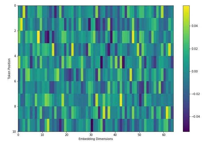
Next, let's look at the Attention in ViT, which should be consistent with the self Attention in Transformer. Let's see how reference [1] introduces self Attention. Reference [1] gives an example of semantic processing
"The animal didn't cross the street because it was too tired."
It is easy for us to understand that the latter it refers to animal, but how can machines associate it with animal?
Self attention is generated under this demand. As shown in the figure above, we should have a structure that can express the relationship between each word and each other word. Here we deal with the image problem. The existence of self attention can be understood as that we should have a structure that can express the relationship between each patch and other patches. As mentioned earlier, the patch in the image can be viewed in the same way as the word in semantic processing.
Let's look at the specific implementation:
1. Create three vectors based on the input vector: query vector, key vector and value vector.
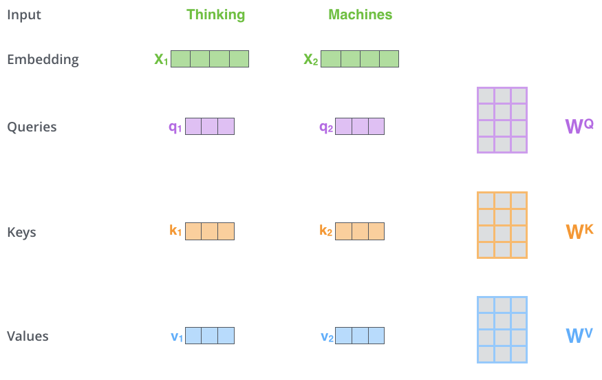
2. Self attention is generated by query vector and key vector.
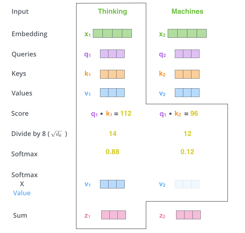
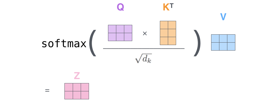
Thinking and Machine can be understood as two patch es in which the picture is segmented. Now calculate the self attention of thinking by multiplying q by k and dividing by a certain coefficient (the result value obtained from the scaled dot product attention is usually large, so that the softmax result can not express the attention value well. At this time, dividing by a scaling factor can alleviate this situation to a certain extent), After passing softmax, you will get an attention vector about thinking. For example, this example is [0.88, 0.12]. This vector means that to explain the meaning of the word thinking in this sentence, you should take 0.88 original meaning of thinking and 0.12 original meaning of Machine, which is the meaning of thinking in this sentence. Finally, the result after Sum in the figure expresses the meaning of each word in this sentence. The whole process can be expressed in the following figure:
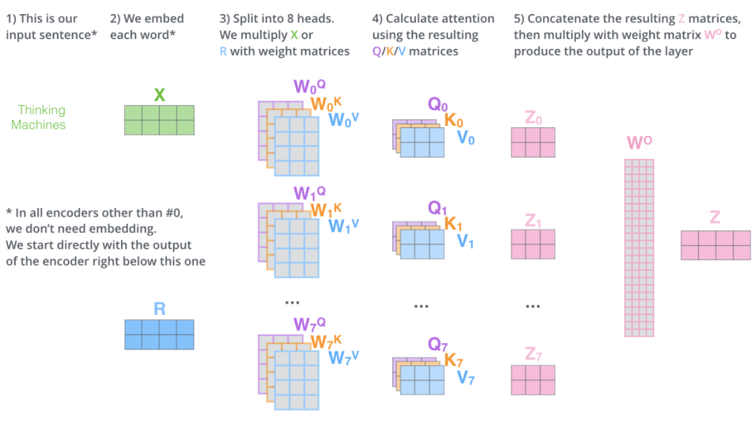
4. Multi-Head Attention
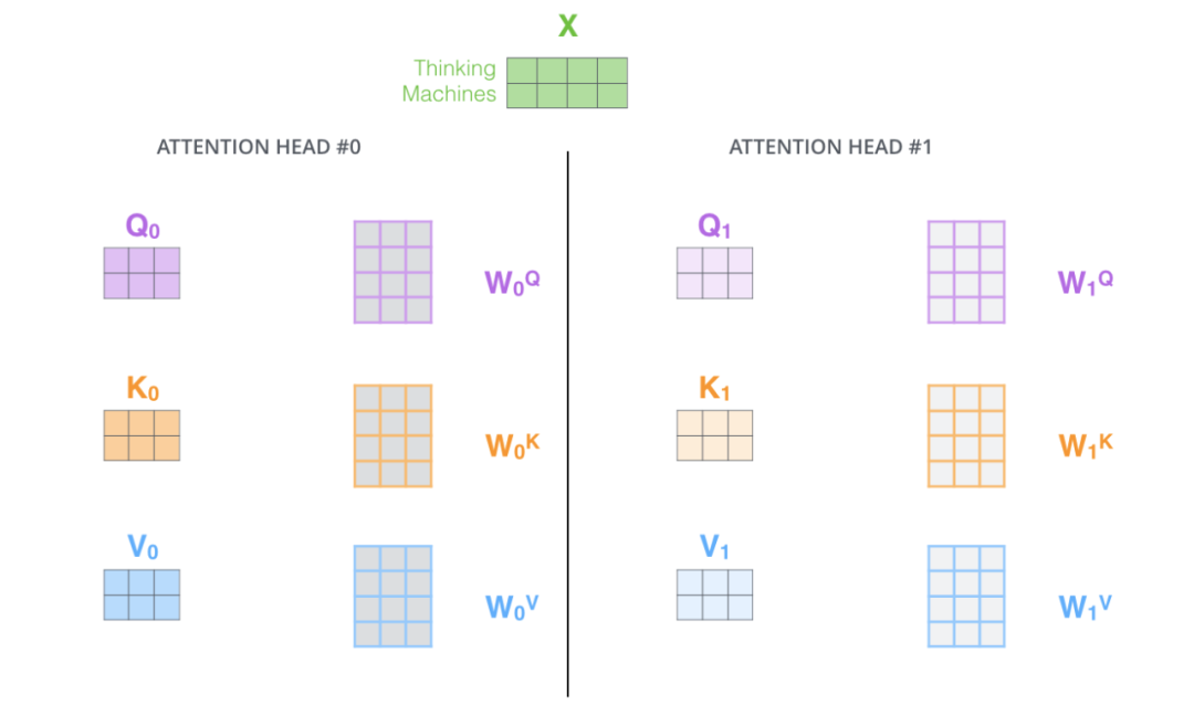
In timm, attention is an improved multi head attention based on self attention, that is, when generating q, k and v, q, k and v are segmented and divided into num_heads, perform self attention operation on each copy respectively, and finally splice them together. In this way, parameter isolation is carried out to a certain extent. As for why the effect is better, I think this operation will concentrate the associated features and make it easier to train.
class Attention(nn.Module):
    def __init__(self, dim, num_heads=8, qkv_bias=False, attn_drop=0., proj_drop=0.):
        super().__init__()
        self.num_heads = num_heads
        #  q. K, V vector length
        head_dim = dim // num_heads
        self.scale = head_dim ** -0.5
        self.qkv = nn.Linear(dim, dim * 3, bias=qkv_bias)
        self.attn_drop = nn.Dropout(attn_drop)
        self.proj = nn.Linear(dim, dim)
        self.proj_drop = nn.Dropout(proj_drop)

    def forward(self, x):
        #  Here C corresponds to E above, the length of the vector
        B, N, C = x.shape
        #  (B, N, C)  ->  (3, B, num_heads, N, C//num_heads), / / means rounding down.
        qkv = self.qkv(x).reshape(B, N, 3, self.num_heads, C // self.num_heads).permute(2, 0, 3, 1, 4)
        #  Cut qkv into three data blocks on the 0 dimension, q,k,v:(B, num_heads,   N,   C//num_heads)
        #  The effect here is to generate three vectors from each vector, namely query, key and value
        q, k, v = qkv.unbind(0)   # make torchscript happy (cannot use tensor as tuple)
        # @ Matrix multiplication to obtain score   (B,num_heads,N,N)
        attn = (q @ k.transpose(-2, -1)) * self.scale
        attn = attn.softmax(dim=-1)
        attn = self.attn_drop(attn)
        # (B,num_heads,N,N)@(B,num_heads,N,C//num_heads)->(B,num_heads,N,C//num_heads)
        # (B,num_heads,N,C//num_heads) ->(B,N,num_heads,C//num_heads)
        # (B,N,num_heads,C//num_heads) -> (B, N, C)
        x = (attn @ v).transpose(1, 2).reshape(B, N, C)
        # (B, N, C) -> (B, N, C)
        x = self.proj(x)
        x = self.proj_drop(x)
        return x
The general diagram of multi head attention is as follows:
5. Layer Normalization
A concept corresponding to Layer normalization is the familiar Batch Normalization. The fundamental difference between the two is that Layer normalization normalizes all features of each sample, while Batch Normalization normalizes all samples of each channel.
For ease of understanding, here is the sample code posted to LN on the official website:
# NLP Example
batch, sentence_length, embedding_dim = 20, 5, 10
embedding = torch.randn(batch, sentence_length, embedding_dim)
#  Specifies the normalized dimension
layer_norm = nn.LayerNorm(embedding_dim)
# Normalization
layer_norm(embedding)

# Image Example
N, C, H, W = 20, 5, 10, 10
input = torch.randn(N, C, H, W)
# Normalize over the last three dimensions (i.e. the channel and spatial dimensions)
# as shown in the image below
layer_norm = nn.LayerNorm([C, H, W])
output = layer_norm(input)
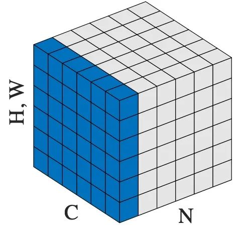
In ViT, although ln processes picture data, before LN, the picture has been cut into patches, and each Patch represents a word. Therefore, it is using semantic logic to solve visual problems. Therefore, LN is also used according to semantic logic in ViT. For details of this concept, please refer to [3] and [2].
6. Drop Path
Dropout is the earliest method used to solve network over fitting and the ancestor of all drop methods. The schematic diagram of the method is as follows:
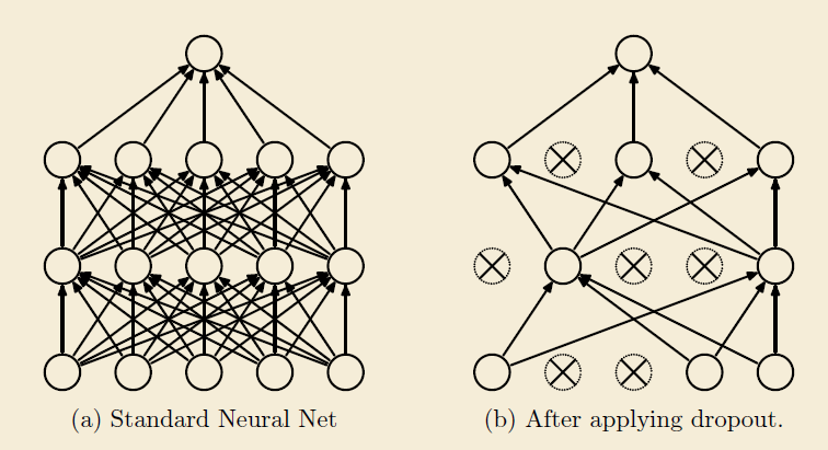
When propagating forward, let the neuron stop working with a certain probability. This can strengthen the generalization ability of the model, because neurons will fail with a certain probability, and such a mechanism will make the results not too dependent on individual neurons. Training phase to keep_prob probability makes neurons fail, and the validity of all neurons will be preserved during reasoning. Therefore, the reasoning result of neurons with dropout added during training should be multiplied by keep_prob.
Next, use the idea of dropout to understand the drop path. If the schematic diagram of drop path is not found, look directly at the code on timm:
def drop_path(x, drop_prob: float = 0., training: bool = False):
    if drop_prob == 0. or not training:
        return x
    #  drop_prob is the probability of droppath
    keep_prob = 1 - drop_prob
    # work with diff dim tensors, not just 2D ConvNets
    #  In ViT, shape is (B, 1,1), and B is batch size
    shape = (x.shape[0],) + (1,) * (x.ndim - 1)
    #  Press shape to generate a random vector between 0-1 and add keep_prob
    random_tensor = keep_prob + torch.rand(shape, dtype=x.dtype, device=x.device)
    #  Round down, binarize, so random_ The expectation of the probability of 1 in tensor is keep_prob
    random_tensor.floor_()  # binarize
    #  Change a certain layer to 0
    output = x.div(keep_prob) * random_tensor
    return output
As can be seen from the code, drop path is to change some layers into 0 at random in the dimension of batch to speed up the operation.
7. Encoder
Transformer architecture diagram:
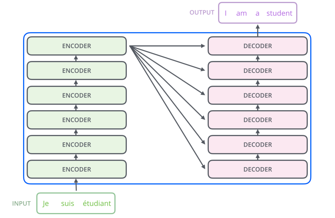
The Transformer is formed by a pile of encoders and decoder s. The general architecture diagram of the encoder is as follows:
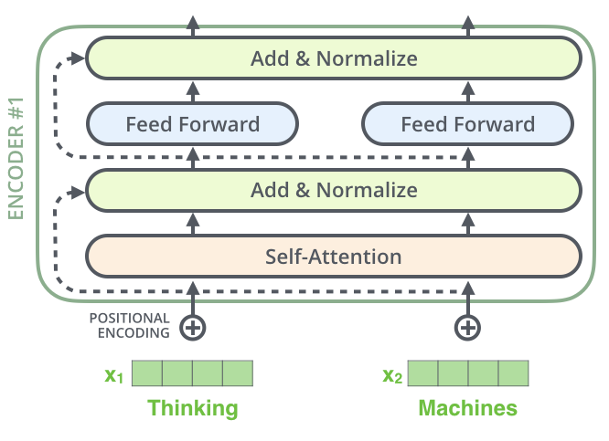
The implementation details of Encoder in ViT are shown in the following code (layer normalization - > multi head attention - > drop path - > Layer normalization - > MLP - > drop path). It is renamed block:
class Block(nn.Module):

    def __init__(self, dim, num_heads, mlp_ratio=4., qkv_bias=False, drop=0., attn_drop=0.,
                 drop_path=0., act_layer=nn.GELU, norm_layer=nn.LayerNorm):
        super().__init__()
        #  Normalize the eigenvector of each channel of each sample
        #  That is, each eigenvector is normalized independently
        # Although we have image data here, the image is cut into patch es using semantic logic
        self.norm1 = norm_layer(dim)
        self.attn = Attention(dim, num_heads=num_heads, qkv_bias=qkv_bias, attn_drop=attn_drop, proj_drop=drop)
        # NOTE: drop path for stochastic depth, we shall see if this is better than dropout here
        self.drop_path = DropPath(drop_path) if drop_path > 0. else nn.Identity()
        self.norm2 = norm_layer(dim)
        mlp_hidden_dim = int(dim * mlp_ratio)
        #  Full connection, excitation, drop, full connection, drop, if out_ If features is not filled in, the output dimension remains unchanged.
        self.mlp = Mlp(in_features=dim, hidden_features=mlp_hidden_dim, act_layer=act_layer, drop=drop)

    def forward(self, x):
        #  Finally, one-dimensional normalization, multi head   attention,   drop_path
        # (B, N, C) -> (B, N, C)
        x = x + self.drop_path(self.attn(self.norm1(x)))
        # (B, N, C) -> (B, N, C)
        x = x + self.drop_path(self.mlp(self.norm2(x)))
        return x
In ViT, such blocks have several layers to form blocks:
# stochastic depth decay rule
dpr = [x.item() for x in torch.linspace(0, drop_path_rate, depth)]
self.blocks = nn.Sequential(*[
    Block(
        dim=embed_dim, num_heads=num_heads, mlp_ratio=mlp_ratio, qkv_bias=qkv_bias, drop=drop_rate,
        attn_drop=attn_drop_rate, drop_path=dpr[i], norm_layer=norm_layer, act_layer=act_layer)
    for i in range(depth)])
If drop_path_ If the rate is greater than 0, the drop of each layer block_ Path increases linearly. Depth is the number of blocks in a block. It can also be understood as the depth of the network block blocks.
8. Forward Features
Patch embedding - > adding CLS - > adding POS embedding - > encoding with blocks - > Layer normalization - > embedding of output graph
def forward_features(self, x):
    #  x by (B, C, H, W) - > (B, N, E)
    x = self.patch_embed(x)
    # stole cls_tokens impl from Phil Wang, thanks
    #  cls_ The token consists of (1,   1,   768)->(B,   1,   768),   B is batch_size
    cls_token = self.cls_token.expand(x.shape[0], -1, -1)
    # dist_ Dist is only used in deit models when token is none_ token.
    if self.dist_token is None:
        #  x by (B,   N,   E)->(B,   1+N,   E)
        x = torch.cat((cls_token, x), dim=1)
    else:
        #  x by (B,   N,   E)->(B,   2+N,   E)
        x = torch.cat((cls_token, self.dist_token.expand(x.shape[0], -1, -1), x), dim=1)
    # + pos_embed:(1,   1+N,   E) , add a dropout layer
    x = self.pos_drop(x + self.pos_embed)
    x = self.blocks(x)
    # nn.LayerNorm
    x = self.norm(x)
    if self.dist_token is None:
        #  Not DeiT, the output is x[:,0], (B,   1,   768), i.e. cls_token
        return self.pre_logits(x[:, 0])
    else:
        #  It's DeiT, and the output is cls_token and dist_token
        return x[:, 0], x[:, 1]
Here, a CLS is added to the dimension of patch_ Token, this existence can be understood in this way. Other embedding express the characteristics of different patches, while cls_token is to synthesize the information of all patches and generate a new embedding to express the information of the whole graph. And dist_token is the structure of DeiT network.
9. Forward
This is the general process of the model: forward features - > final output
    def forward(self, x):
        #(B,C,H,W)-> (B, 1, 768)
        # (B,C,H,W) -> (B, 1, 768), (B, 1, 768)
        x = self.forward_features(x)

        if self.head_dist is not None:
            #  If num_ classes>0,   (B,   1,   768)->(B,   1,   num_classes)
            # Otherwise unchanged
            x, x_dist = self.head(x[0]), self.head_dist(x[1])
            if self.training and not torch.jit.is_scripting():
                return x, x_dist
            else:
                # during inference,
                # return the average of both classifier predictions
                return (x + x_dist) / 2
        else:
            #  If num_ classes>0, (B,   1,   768)->(B,   1,   num_classes)
            #  Otherwise unchanged
            x = self.head(x)
        return x
In this way, ViT is finished for me. DeiT involves many new concepts. Later, we will refer to the code for detailed explanation.

Feel useful, pay attention, watch, like, forward and share a wave!
