Tensorflow 2.0 - FaceNet network principle and code analysis (I) - model principle and backbone network

FaceNet is actually a general face recognition system described in the preface: deep convolution neural network (CNN) is used to map images to European space. Spatial distance is directly related to image similarity: different images of the same person have a small spatial distance, and images of different people have a large spatial distance, which can be used for face verification, recognition and clustering. After training with 8 million people and more than 200 million sample sets, the accuracy rate of FaceNet on LFW dataset is 99.63%, and that on YouTube Faces DB dataset is 95.12%.

code: FaceNet

1, Algorithm principle

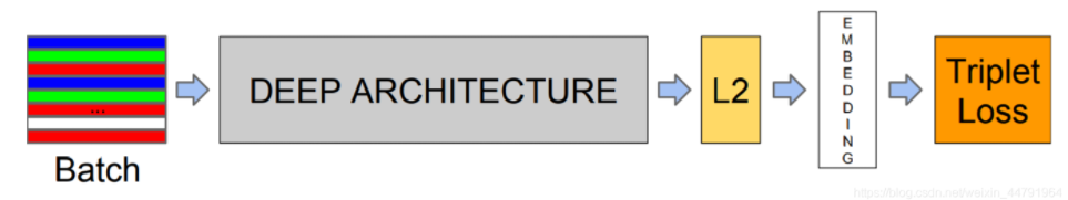
The figure above shows the general framework of facenet. It can be seen that a batch training image is extracted through a black box. Among them, DEEP ARCHITECTURE is generally a mature backbone. The earliest facenet adopted two kinds of deep convolution networks: the classic Zeiler & Ferguson architecture and Google's concept v1. The latest facenet has been improved. The main model adopts a very deep network Inception ResNet -v2, which is composed of three Inception modules with residual connection and one Inception v4 module. mobilenet or Inception is usually used in code implementation_ Resnetv1 acts as the backbone network.
After feature extraction, L2 standardization is carried out, and then a 128 dimensional vector is obtained.
Finally, triple loss calculation is performed.

Next, it will be introduced according to each module~

2, Backbone network

Here, we choose mobilenet as the backbone network.
In the code, backbone = "mobilenet", and then substitute model = facent (input_shape, num_classes, backbone = backbone, mode = "train"), all the codes implemented by mobilenet are in nets/mobilenet.py.

def _conv_block(inputs, filters, kernel=(3, 3), strides=(1, 1)):
    x = Conv2D(filters, kernel,
               padding='same',
               use_bias=False,
               strides=strides,
               name='conv1')(inputs)
    x = BatchNormalization(name='conv1_bn')(x)
    return Activation(relu6, name='conv1_relu')(x)

This is a typical convolution BN activation module. There's nothing to say~

def _depthwise_conv_block(inputs, pointwise_conv_filters, depth_multiplier=1, strides=(1, 1), block_id=1):
    x = DepthwiseConv2D((3, 3),
                        padding='same',
                        depth_multiplier=depth_multiplier,
                        strides=strides,
                        use_bias=False,
                        name='conv_dw_%d' % block_id)(inputs)

    x = BatchNormalization(name='conv_dw_%d_bn' % block_id)(x)
    x = Activation(relu6, name='conv_dw_%d_relu' % block_id)(x)

    x = Conv2D(pointwise_conv_filters, (1, 1),
               padding='same',
               use_bias=False,
               strides=(1, 1),
               name='conv_pw_%d' % block_id)(x)
    x = BatchNormalization(name='conv_pw_%d_bn' % block_id)(x)
    return Activation(relu6, name='conv_pw_%d_relu' % block_id)(x)

This module is different from the above modules because it contains a depthwise conv2d. The difference between it and the ordinary conv2d is that conv2d convolutes at each depth, then sums and depthwise_conv2d convolution, no sum.
For details, please refer to: https://blog.csdn.net/u010879745/article/details/108043183

def MobileNet(inputs, embedding_size=128, dropout_keep_prob=0.4, alpha=1.0, depth_multiplier=1):
    # 160,160,3 -> 80,80,32
    x = _conv_block(inputs, 32, strides=(2, 2))
    
    # 80,80,32 -> 80,80,64
    x = _depthwise_conv_block(x, 64, depth_multiplier, block_id=1)

    # 80,80,64 -> 40,40,128
    x = _depthwise_conv_block(x, 128, depth_multiplier, strides=(2, 2), block_id=2)
    x = _depthwise_conv_block(x, 128, depth_multiplier, block_id=3)

    # 40,40,128 -> 20,20,256
    x = _depthwise_conv_block(x, 256, depth_multiplier, strides=(2, 2), block_id=4)
    x = _depthwise_conv_block(x, 256, depth_multiplier, block_id=5)

    # 20,20,256 -> 10,10,512
    x = _depthwise_conv_block(x, 512, depth_multiplier, strides=(2, 2), block_id=6)
    x = _depthwise_conv_block(x, 512, depth_multiplier, block_id=7)
    x = _depthwise_conv_block(x, 512, depth_multiplier, block_id=8)
    x = _depthwise_conv_block(x, 512, depth_multiplier, block_id=9)
    x = _depthwise_conv_block(x, 512, depth_multiplier, block_id=10)
    x = _depthwise_conv_block(x, 512, depth_multiplier, block_id=11)

    # 10,10,512 -> 5,5,1024
    x = _depthwise_conv_block(x, 1024, depth_multiplier, strides=(2, 2), block_id=12)
    x = _depthwise_conv_block(x, 1024, depth_multiplier, block_id=13)
    
    # 1024
    x = GlobalAveragePooling2D()(x)
    # Prevent the network from over fitting and play a role in training
    x = Dropout(1.0 - dropout_keep_prob, name='Dropout')(x)
    # Full connection layer to 128
    # 128
    x = Dense(embedding_size, use_bias=False, name='Bottleneck')(x)
    x = BatchNormalization(momentum=0.995, epsilon=0.001, scale=False,
                           name='BatchNorm_Bottleneck')(x)
 
    # Create model
    model = Model(inputs, x, name='mobilenet')

    return model

The above is the network structure of mobilenet. It can be seen that the implementation is very simple and clear. After the input picture of (160160,3) passes through DEEP ARCHITECTURE, a (5,51024) feature map is generated, and then a global average pooling 2D (global average pooling) is carried out, GAP introduction In this blog, I made a brief introduction to GAP. The GAP layer changes (5,51024) into (1,11024), and then makes a Dropout. Finally, connect a fully connected layer and change it into a vector with a length of 128.