1 Preface

Hi, everyone, this is senior Dan Cheng. Today, I'm doing an e-commerce sales forecast analysis. This is just a demo. I'm trying to analyze the film data and visualize the system

Bi design help, problem opening guidance, technical solutions
🇶746876041

2 principle of spam SMS / Email Classification Algorithm

Spam content is often advertising or false information, even bad information such as computer virus, erotic, reactionary and so on. The existence of a large number of spam will not only bring trouble to people, but also cause a waste of network resources;

Network public opinion is a form of social public opinion. Network public opinion has the characteristics of rapid formation, great influence and strong organizational advantages. The quality of network public opinion has a great impact on social stability. Improving the ability of public opinion analysis to effectively obtain the nature of public opinion and avoid the adverse impact of negative public opinion is a serious topic facing the Internet.

E-mail is divided into spam (harmful information) and normal e-mail. Network public opinion is divided into negative public opinion (harmful information) and positive public opinion. Then, both spam filtering and network public opinion analysis can be regarded as the two classification problem of short text.

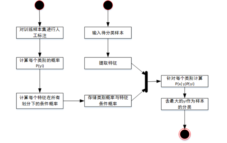
2.1 commonly used classifier - Bayesian classifier

Bayesian algorithm solves a typical problem in probability theory: there are 20 red balls and 20 white balls in box 1, 10 oil white balls and 30 red balls in box 2. Now select a box randomly and take out a ball whose color is red. What is the probability that the ball comes from box 1?

The Bayesian algorithm is used to identify spam. Based on the same principle, the probability of a group of eigenvalues is obtained according to the classified basic information (such as the probability of the word "tea" appearing in spam and the probability of non spam), the classification model is obtained, and then the eigenvalues are extracted from the information to be processed, combined with the classification model to judge its classification.

Bayesian formula:

P(B|A)=P(A|B)*P(B)/P(A)

P(B|A) = what is the probability of B when condition A occurs. Substitute: when the ball is red, what is the probability of coming from box 1?

P(A|B) = probability of taking out the red ball when box 1 is selected.

P(B) = probability of box 1.

P(A) = probability of taking out the red ball.

Substitute spam identification:

P(B|A) = what is the probability of spam when the word "tea" is included?

P(A|B) = what is the probability of including the word "tea" when the email is spam?

P(B) = total probability of spam.

P(A) = probability that "tea" appears in all eigenvalues.

3 data set introduction

Use the Chinese mail data set: Senior Dan Cheng collected it by himself, through crawler and manual screening.

The dataset is in the "data" folder, including the "full" folder and the "delay" folder.

The "data" folder contains multiple secondary folders. The spam text is in the secondary folder, and one text represents an email. There is an index file in the "full" folder, which records the labels of each mail text.

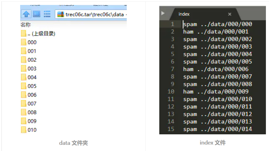
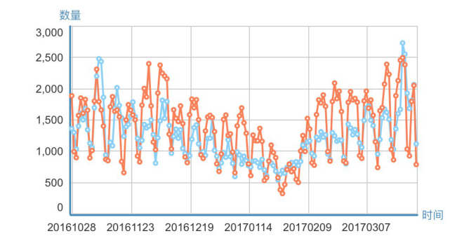
Dataset visualization:

4 data preprocessing

In this step, the mail samples and sample labels will be extracted into a separate file, and the non Chinese characters of the mail will be removed to divide the mail into good words.

The general contents of the email are as follows:

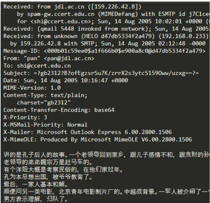
In addition to the email text, each email sample also contains other information, such as sender's mailbox, recipient's mailbox, etc. Because I want to classify spam simply as a text classification task, I ignore this information here.
Read the mail samples in all directories recursively, and write them into a text after dividing the words with jieba. A line of text represents a mail sample:

import re
import jieba
import codecs
import os 
# Remove non Chinese characters
def clean_str(string):
    string = re.sub(r"[^\u4e00-\u9fff]", " ", string)
    string = re.sub(r"\s{2,}", " ", string)
    return string.strip()

def get_data_in_a_file(original_path, save_path='all_email.txt'):
    files = os.listdir(original_path)
    for file in files:
        if os.path.isdir(original_path + '/' + file):
                get_data_in_a_file(original_path + '/' + file, save_path=save_path)
        else:
            email = ''
            # Be careful to use 'ignore', otherwise an error will be reported
            f = codecs.open(original_path + '/' + file, 'r', 'gbk', errors='ignore')
            # lines = f.readlines()
            for line in f:
                line = clean_str(line)
                email += line
            f.close()
            """
            Discovery is used in recursion 'a' The mode of writing files one by one is better than using it once after recursion 'w' Mode writes files much faster
            """
            f = open(save_path, 'a', encoding='utf8')
            email = [word for word in jieba.cut(email) if word.strip() != '']
            f.write(' '.join(email) + '\n')

print('Storing emails in a file ...')
get_data_in_a_file('data', save_path='all_email.txt')
print('Store emails finished !')

Then write the sample label to a separate file, 0 for spam and 1 for non spam. The code is as follows:

def get_label_in_a_file(original_path, save_path='all_email.txt'):
    f = open(original_path, 'r')
    label_list = []
    for line in f:
        # spam
        if line[0] == 's':
            label_list.append('0')
        # ham
        elif line[0] == 'h':
            label_list.append('1')

    f = open(save_path, 'w', encoding='utf8')
    f.write('\n'.join(label_list))
    f.close()

print('Storing labels in a file ...')
get_label_in_a_file('index', save_path='label.txt')
print('Store labels finished !')

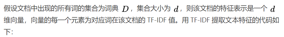
5 feature extraction

This paper uses TF-IDF method to convert text data into numerical data.

TF-IDF is term frequency, Inverse Document Frequency. The formula is as follows:

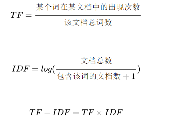
In all documents, the IDF of a word is the same, and the TF is different. In a document, the higher the TF and IDF of a word, it indicates that the word appears more in the document and less in other documents. Therefore, the word is of high importance to this document and can be used to distinguish this document.

import jieba
from sklearn.feature_extraction.text import TfidfVectorizer

def tokenizer_jieba(line):
    # Stutter participle
    return [li for li in jieba.cut(line) if li.strip() != '']

def tokenizer_space(line):
    # Word segmentation by space
    return [li for li in line.split() if li.strip() != '']

def get_data_tf_idf(email_file_name):
    # The mail sample has been divided into words, which are separated by spaces, so tokenizer=tokenizer_space
    vectoring = TfidfVectorizer(input='content', tokenizer=tokenizer_space, analyzer='word')
    content = open(email_file_name, 'r', encoding='utf8').readlines()
    x = vectoring.fit_transform(content)
    return x, vectoring

6 training classifier

Here is a simple example of a logistic regression classifier

from sklearn.linear_model import LogisticRegression
from sklearn import svm, ensemble, naive_bayes
from sklearn.model_selection import train_test_split
from sklearn import metrics
import numpy as np

if __name__ == "__main__":
    np.random.seed(1)
    email_file_name = 'all_email.txt'
    label_file_name = 'label.txt'
    x, vectoring = get_data_tf_idf(email_file_name)
    y = get_label_list(label_file_name)

    # print('x.shape : ', x.shape)
    # print('y.shape : ', y.shape)
    
    # Randomly disrupt all samples
    index = np.arange(len(y))  
    np.random.shuffle(index)
    x = x[index]
    y = y[index]

    # Divide training set and test set
    x_train, x_test, y_train, y_test = train_test_split(x, y, test_size=0.2)

    clf = svm.LinearSVC()
    # clf = LogisticRegression()
    # clf = ensemble.RandomForestClassifier()
    clf.fit(x_train, y_train)
    y_pred = clf.predict(x_test)
    print('classification_report\n', metrics.classification_report(y_test, y_pred, digits=4))
    print('Accuracy:', metrics.accuracy_score(y_test, y_pred))

7 comprehensive test results

2000 pieces of data were tested using the following methods:

• Support vector machine SVM

• Random number deep forest

• logistic regression
  

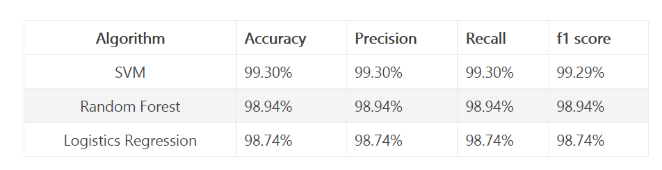
It can be seen that the accuracy of 2000 data training results and 200 test results is still high, but there are few data, which is difficult to explain the problem.

8 other model methods

You can also build a deep learning model

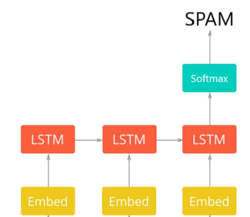
The first layer of the network architecture is the pre trained embedding layer, which maps each word to the N-dimensional vector of the real number (EMBEDDING_SIZE corresponds to the size of the vector, in this case 100). Two words with similar meanings often have very close vectors.

The second layer is a recurrent neural network with LSTM units. Finally, the output layer consists of two neurons, each corresponding to "spam" or "normal mail" with softmax activation function.

def get_embedding_vectors(tokenizer, dim=100):
embedding_index = {}
with open(f"data/glove.6B.{dim}d.txt", encoding='utf8') as f:
for line in tqdm.tqdm(f, "Reading GloVe"):
values = line.split()
word = values[0]
vectors = np.asarray(values[1:], dtype='float32')
embedding_index[word] = vectors

word_index = tokenizer.word_index
embedding_matrix = np.zeros((len(word_index)+1, dim))
for word, i in word_index.items():
embedding_vector = embedding_index.get(word)
if embedding_vector is not None:
# words not found will be 0s
embedding_matrix[i] = embedding_vector

return embedding_matrix

def get_model(tokenizer, lstm_units):
"""
Constructs the model,
Embedding vectors => LSTM => 2 output Fully-Connected neurons with softmax activation
"""
# get the GloVe embedding vectors
embedding_matrix = get_embedding_vectors(tokenizer)
model = Sequential()
model.add(Embedding(len(tokenizer.word_index)+1,
EMBEDDING_SIZE,
weights=[embedding_matrix],
trainable=False,
input_length=SEQUENCE_LENGTH))

model.add(LSTM(lstm_units, recurrent_dropout=0.2))
model.add(Dropout(0.3))
model.add(Dense(2, activation="softmax"))
# compile as rmsprop optimizer
# aswell as with recall metric
model.compile(optimizer="rmsprop", loss="categorical_crossentropy",
metrics=["accuracy", keras_metrics.precision(), keras_metrics.recall()])
model.summary()
return model

The training results are as follows:

_________________________________________________________________
Layer (type) Output Shape Param #
=================================================================
embedding_1 (Embedding) (None, 100, 100) 901300
_________________________________________________________________
lstm_1 (LSTM) (None, 128) 117248
_________________________________________________________________
dropout_1 (Dropout) (None, 128) 0
_________________________________________________________________
dense_1 (Dense) (None, 2) 258
=================================================================
Total params: 1,018,806
Trainable params: 117,506
Non-trainable params: 901,300
_________________________________________________________________
X_train.shape: (4180, 100)
X_test.shape: (1394, 100)
y_train.shape: (4180, 2)
y_test.shape: (1394, 2)
Train on 4180 samples, validate on 1394 samples
Epoch 1/20
4180/4180 [==============================] - 9s 2ms/step - loss: 0.1712 - acc: 0.9325 - precision: 0.9524 - recall: 0.9708 - val_loss: 0.1023 - val_acc: 0.9656 - val_precision: 0.9840 - val_recall: 0.9758

Epoch 00001: val_loss improved from inf to 0.10233, saving model to results/spam_classifier_0.10
Epoch 2/20
4180/4180 [==============================] - 8s 2ms/step - loss: 0.0976 - acc: 0.9675 - precision: 0.9765 - recall: 0.9862 - val_loss: 0.0809 - val_acc: 0.9720 - val_precision: 0.9793 - val_recall: 0.9883

9 finally - design help

Bi design help, problem opening guidance, technical solutions
🇶746876041