Scikit learn is a very beautiful one machine learning Libraries. Sometimes, using these libraries can save you a lot of time. At least, we can use them Python , it should be difficult to write such fast code

Scikit learn has some official documents, but personally, I don't think many things in its documents are clear. When it says the principle of the algorithm, it just describes it. Unless you are familiar with the algorithm, you will smile at its description. When it describes the API, it often only talks about some common usages, and some more advanced usages are vague, Although many people say that the document of this thing is well written, I think it's a special pit. So this blog will record some pits I encountered when using this library and how to cross them. Update it slowly. Of course, if it's not used in the future, the article will not be updated. Of course, I don't intend to say how many people can read this article. That's it

clustering

Pit 1: how to customize the distance function?

Although the scikit learn library implements many clustering functions, most of the distances used by these algorithms are Euclidean distance or Minkowski distance. In fact, according to the description in our textbook, the so-called distance is not the only two. For different purposes, we can use different distances to measure the distance between two vectors, but unfortunately, I didn't see the option to customize the distance in scikit learn. I searched all over the Internet and didn't see it

But don't worry, we can implement this indirectly. Take the DBSCAN algorithm as an example, here is a constructor of the class:

class sklearn.cluster.DBSCAN(eps=0.5, min_samples=5, metric='euclidean', algorithm='auto', leaf_size=30, p=None, n_jobs=1)
# eps represents the maximum distance that two vectors can be regarded as the same class
# min_samples indicates at least the number of elements to be included in a class. If it is less than this number, it will not form a class

We should pay special attention to the metric option. Let's take a look at the options:

metric : string, or callable
    The metric to use when calculating distance between instances in a feature array. If metric is a string or callable, it must be one of the options allowed by metrics.pairwise.calculate_distance for its metric parameter. 
    If metric is "precomputed", X is assumed to be a distance matrix and must be square. X may be a sparse matrix, in which case only "nonzero" elements may be considered neighbors for DBSCAN.
    New in version 0.17: metric precomputed to accept precomputed sparse matrix.

This description actually reveals a very important information, that is, you can calculate the similarity of each vector in advance to form a similarity matrix. As long as you set metric='precomputedd ', how to call it?

Let's look at the fit function

fit(X, y=None, sample_weight=None)
# X : array or sparse (CSR) matrix of shape (n_samples, n_features), or array of shape (n_samples, n_samples)
# A feature array, or array of distances between samples if metric='precomputed'.

If you set metric to precomputed, the X parameter passed in should be the similarity matrix between vectors, and then the fit function will directly use your matrix for calculation. Otherwise, you still have to pass in vectors in the form of n_samples, n_features

What does this mean, comrades? That means that we can calculate the similarity of each vector in advance with our custom distance, and then call this function to get the result. Is that very cool?

Specific how to program, I give an example, throw a brick

import numpy as np
from sklearn.cluster import DBSCAN
if __name__ == '__main__':
    Y = np.array([[0, 1, 2],
                  [1, 0, 3],
                  [2, 3, 0]]) # Similarity matrix, the smaller the distance, the closer the distance between the two vectors
    # N = Y.shape[0]
    db = DBSCAN(eps=0.13, metric='precomputed', min_samples=3).fit(Y)
    labels = db.labels_
    # Then take a look at the classification results!
    n_clusters_ = len(set(labels)) - (1 if -1 in labels else 0) # Number of classes
    print('The number of classes is:%d'%(n_clusters_))

Let's continue to look at AP clustering, which is actually very similar:

class sklearn.cluster.AffinityPropagation(damping=0.5, max_iter=200, convergence_iter=15, copy=True, preference=None, affinity='euclidean', verbose=False)

The key lies in this affinity parameter:

affinity : string, optional, default=``euclidean``
    Which affinity to use. At the moment precomputed and euclidean are supported. euclidean uses the negative squared euclidean distance between points.

This thing also supports precomputed parameters. Let's take a look at the fit function:

fit(X, y=None)
# Create affinity matrix from negative euclidean distances, then apply affinity propagation clustering.
# Parameters:   
#   X: array-like, shape (n_samples, n_features) or (n_samples, n_samples) :
#   Data matrix or, if affinity is precomputed, matrix of similarities / affinities.

The X here is similar to the previous one. If you set metric to precomputed, the passed in X parameter should be the similarity matrix between each vector, and then the fit function will directly use your matrix for calculation. Otherwise, you still have to pass in a vector in the form of n_samples, n_features

Example 1

"""
    target:
    ~~~~~~~~~~~~~~~~
    In this file,What I want to test most is,Are my previous clustering algorithms correct.
    The first thing to test is AP clustering.
"""
from sklearn.cluster import AffinityPropagation
from sklearn import metrics
from sklearn.datasets.samples_generator import make_blobs
from sklearn.metrics.pairwise import euclidean_distances
import matplotlib.pyplot as plt
from itertools import cycle

def draw_pic(n_clusters, cluster_centers_indices, labels, X):
    ''' words alone are no proof,Draw a picture at a glance. '''
    colors = cycle('bgrcmykbgrcmykbgrcmykbgrcmyk')
    for k, col in zip(range(n_clusters), colors):
        class_members = labels == k
        cluster_center = X[cluster_centers_indices[k]] # Get the center of the cluster
        plt.plot(X[class_members, 0], X[class_members, 1], col + '.')
        plt.plot(cluster_center[0], cluster_center[1], 'o', markerfacecolor=col,
                 markeredgecolor='k', markersize=14)
        for x in X[class_members]:
            plt.plot([cluster_center[0], x[0]], [cluster_center[1], x[1]], col)

    plt.title('Estimated number of clusters: %d' % n_clusters)
    plt.show()


if __name__ == '__main__':
    centers = [[1, 1], [-1, -1], [1, -1]]
    # Next, 300 points are generated, and the center of each point should be marked and recorded in labels_true
    X, labels_true = make_blobs(n_samples=300, centers=centers,
                                cluster_std=0.5, random_state=0)
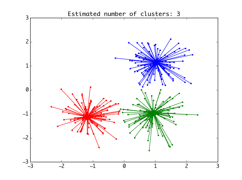
    af = AffinityPropagation(preference=-50).fit(X) # Start clustering with AP
    cluster_centers_indices = af.cluster_centers_indices_ # Get the center point of the cluster
    labels = af.labels_ # Get label
    n_clusters = len(cluster_centers_indices) # Number of classes
    draw_pic(n_clusters, cluster_centers_indices, labels, X)

    #===========Next, calculate the distance in advance=================#
    distance_matrix = -euclidean_distances(X, squared=True) # Calculate the Euclidean distance in advance. It should be noted that the square of Euclidean distance is used here
    af1 = AffinityPropagation(affinity='precomputed', preference=-50).fit(distance_matrix)
    cluster_centers_indices1 = af1.cluster_centers_indices_ # Get the center of the cluster
    labels1 = af1.labels_ # Get label
    n_clusters1 = len(cluster_centers_indices1) # Number of classes
    draw_pic(n_clusters1, cluster_centers_indices1, labels1, X)

Both methods will produce such a diagram:

Example 2

Now that we are here, let's simply test the DBSCAN algorithm

"""
    target:
    ~~~~~~~~~~~~~~
    It's been tested before ap clustering,Next test DBSACN.
"""
import numpy as np
from sklearn.cluster import DBSCAN
from sklearn import metrics
from sklearn.datasets.samples_generator import make_blobs
from sklearn.preprocessing import StandardScaler
import matplotlib.pyplot as plt
from sklearn.metrics.pairwise import euclidean_distances

def draw_pic(n_clusters, core_samples_mask, labels, X):
    ''' Start drawing pictures '''
    # Black removed and is used for noise instead.
    unique_labels = set(labels)
    colors = plt.cm.Spectral(np.linspace(0, 1, len(unique_labels)))
    for k, col in zip(unique_labels, colors):
        if k == -1:
            # Black used for noise.
            col = 'k'

        class_member_mask = (labels == k)

        xy = X[class_member_mask & core_samples_mask]
        plt.plot(xy[:, 0], xy[:, 1], 'o', markerfacecolor=col,
                 markeredgecolor='k', markersize=14)

        xy = X[class_member_mask & ~core_samples_mask]
        plt.plot(xy[:, 0], xy[:, 1], 'o', markerfacecolor=col,
                 markeredgecolor='k', markersize=6)

    plt.title('Estimated number of clusters: %d' % n_clusters)
    plt.show()

if __name__ == '__main__':
    #=========Generate data first===========#
    centers = [[1, 1], [-1, -1], [1, -1]]
    X, labels_true = make_blobs(n_samples=750, centers=centers,
                                cluster_std=0.4, random_state=0)
    X = StandardScaler().fit_transform(X)
    #=========Next, start clustering==========#
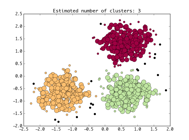
    db = DBSCAN(eps=0.3, min_samples=10).fit(X)
    labels = db.labels_ # Label for each point
    core_samples_mask = np.zeros_like(db.labels_, dtype=bool)
    core_samples_mask[db.core_sample_indices_] = True
    n_clusters = len(set(labels)) - (1 if -1 in labels else 0) # Number of classes
    draw_pic(n_clusters, core_samples_mask, labels, X)
    #==========Next, we calculate the distance in advance============#
    distance_matrix =  euclidean_distances(X)
    db1 = DBSCAN(eps=0.3, min_samples=10, metric='precomputed').fit(distance_matrix)
    labels1 = db1.labels_ # Label for each point
    core_samples_mask1 = np.zeros_like(db1.labels_, dtype=bool)
    core_samples_mask1[db1.core_sample_indices_] = True
    n_clusters1 = len(set(labels1)) - (1 if -1 in labels1 else 0) # Number of classes
    draw_pic(n_clusters1, core_samples_mask1, labels1, X)

Both methods will produce such a diagram:

OK, that's all for now, but interestingly, the simplest KMeans algorithm doesn't support such work