🔥 This article GitHub https://github.com/kzbkzb/Python-AI Included
1. Preface
Today is the 10th day, we will use LSTM to forecast the opening price of the stock. The final R2 will reach 0.74, which is two percentage points higher than the traditional RNN of 0.72.
My environment:
- Language environment: Python 3.6.5
- Compiler: jupyter notebook
- Deep learning environment: TensorFlow2.4.1
- Data and Code: 📌 [Portal]
From column: [100 cases of deep learning]
Previous highlights:
- Hello Word in Deep Learning 100 Cases Convolutional Neural Network (LeNet-5) | Day 22
- 100 Cases of in-depth Learning Convolutional Neural Network (CNN) for mnist Handwritten Number Recognition|Day 1
- Deep Learning 100 Cases-Convolution Neural Network (CNN) Clothing Image Classification|Day 3
- 100 in-depth learning - convolution neural network (CNN) flower recognition | Day 4
- In-depth Learning 100 Cases-Convolutional Neural Network (CNN) Weather Identification|Day 5
- Deep Learning 100 Cases-Convolutional Neural Network (VGG-16) Identify a gang of squid caps|Day 6
- Deep Learning 100 Cases-Convolutional Neural Network (ResNet-50) Bird Identification|Day 8
- In-depth Learning 100 Cases-Circulating Neural Network (RNN) Stock Forecasting|Day 9
If you're still a little white, take a look at this special column I wrote for you: "Beginning with Little White Deep Learning" To help you get started with zero basics.
2. What is LSTM
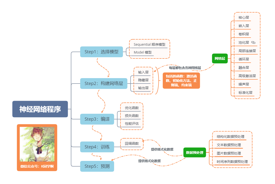
Basic Processes of Neural Network Programs
One sentence introduces LSTM, which is an advanced version of RNN. If the maximum extent of RNN is to understand a sentence, then the maximum extent of LSTM is to understand a sentence, described in detail as follows:
LSTM, all known as Long Short Term Memory networks, is a special RNN that learns long-term dependencies. LSTM was proposed by Hochreiter & Schmidhuber (1997), and many researchers have done a series of work to improve and promote it. LSTM works well on many issues and is now widely used.
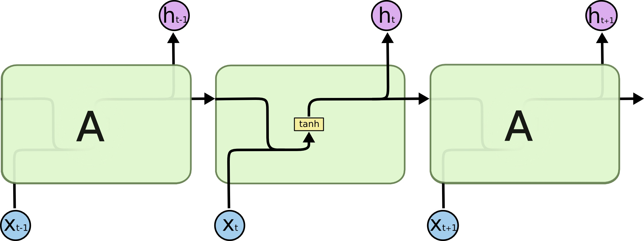
All recurrent neural networks have chains of repetitive neural network modules. In ordinary RNs, the repeat module structure is very simple, and its structure is as follows:
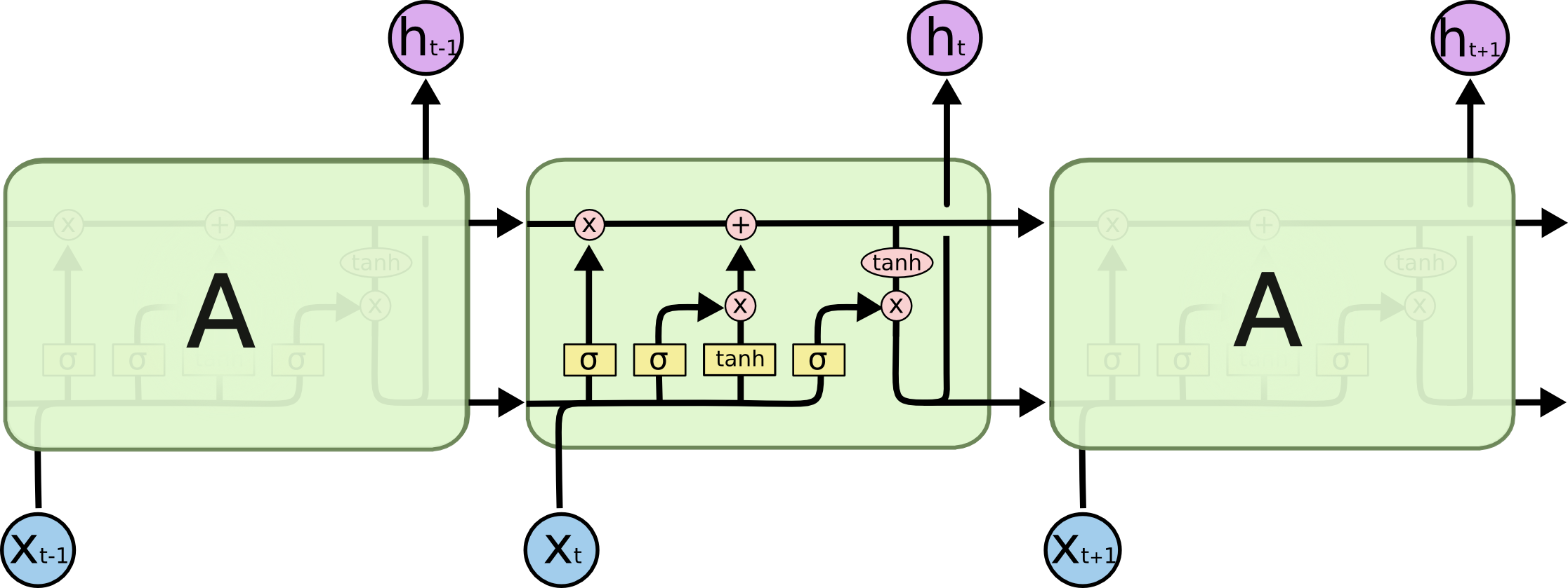
LSTM avoids long-term dependency. You can remember long-term information! LSTM has a more complex structure inside. You can choose to adjust the transmitted information through the gated state, remember the information that needs to be remembered for a long time, and forget the information that is not important. The structure is as follows:
3. Preparations
1. Set up GPU
If you are using a CPU, you can comment out this part of the code.
import tensorflow as tf

gpus = tf.config.list_physical_devices("GPU")

if gpus:
    tf.config.experimental.set_memory_growth(gpus[0], True)  #Set GPU display memory usage on demand
    tf.config.set_visible_devices([gpus[0]],"GPU")
2. Set up related parameters
import pandas            as pd
import tensorflow        as tf
import numpy             as np
import matplotlib.pyplot as plt
# Support Chinese
plt.rcParams['font.sans-serif'] = ['SimHei']  # Used for normal display of Chinese labels
plt.rcParams['axes.unicode_minus'] = False  # Used for normal negative sign display

from numpy                 import array
from sklearn               import metrics
from sklearn.preprocessing import MinMaxScaler
from keras.models          import Sequential
from keras.layers          import Dense,LSTM,Bidirectional


# Ensure results are as reproducible as possible
from numpy.random          import seed
seed(1)
tf.random.set_seed(1)

# Set related parameters
n_timestamp  = 40    # time stamp
n_epochs     = 20    # Number of training rounds
# ====================================
#      Select a model:
#            1:Single Layer LSTM
#            2:Multilayer LSTM
#            3:Bidirectional LSTM
# ====================================
model_type = 1
3. Loading data
data = pd.read_csv('./datasets/SH600519.csv')  # Read stock file

data
| Unnamed: 0 | date | open | close | high | low | volume | code | |
|---|---|---|---|---|---|---|---|---|
| 0 | 74 | 2010-04-26 | 88.702 | 87.381 | 89.072 | 87.362 | 107036.13 | 600519 |
| 1 | 75 | 2010-04-27 | 87.355 | 84.841 | 87.355 | 84.681 | 58234.48 | 600519 |
| 2 | 76 | 2010-04-28 | 84.235 | 84.318 | 85.128 | 83.597 | 26287.43 | 600519 |
| 3 | 77 | 2010-04-29 | 84.592 | 85.671 | 86.315 | 84.592 | 34501.20 | 600519 |
| 4 | 78 | 2010-04-30 | 83.871 | 82.340 | 83.871 | 81.523 | 85566.70 | 600519 |
| ... | ... | ... | ... | ... | ... | ... | ... | ... |
| 2421 | 2495 | 2020-04-20 | 1221.000 | 1227.300 | 1231.500 | 1216.800 | 24239.00 | 600519 |
| 2422 | 2496 | 2020-04-21 | 1221.020 | 1200.000 | 1223.990 | 1193.000 | 29224.00 | 600519 |
| 2423 | 2497 | 2020-04-22 | 1206.000 | 1244.500 | 1249.500 | 1202.220 | 44035.00 | 600519 |
| 2424 | 2498 | 2020-04-23 | 1250.000 | 1252.260 | 1265.680 | 1247.770 | 26899.00 | 600519 |
| 2425 | 2499 | 2020-04-24 | 1248.000 | 1250.560 | 1259.890 | 1235.180 | 19122.00 | 600519 |
2426 rows × 8 columns
"""
Front(2426-300=2126)Day's opening price as training set,Opening price in the next 300 days as test set
"""
training_set = data.iloc[0:2426 - 300, 2:3].values
test_set     = data.iloc[2426 - 300:, 2:3].values
4. Data Preprocessing
1. Normalization
#Normalize data in a range of 0 to 1
sc  = MinMaxScaler(feature_range=(0, 1))
training_set_scaled = sc.fit_transform(training_set)
testing_set_scaled  = sc.transform(test_set)
2. Timestamp function
# N_before taking The data for timestamp days is X; N_ Timstamp+1 day data is Y.
def data_split(sequence, n_timestamp):
    X = []
    y = []
    for i in range(len(sequence)):
        end_ix = i + n_timestamp

        if end_ix > len(sequence)-1:
            break

        seq_x, seq_y = sequence[i:end_ix], sequence[end_ix]
        X.append(seq_x)
        y.append(seq_y)
    return array(X), array(y)

X_train, y_train = data_split(training_set_scaled, n_timestamp)
X_train          = X_train.reshape(X_train.shape[0], X_train.shape[1], 1)

X_test, y_test   = data_split(testing_set_scaled, n_timestamp)
X_test           = X_test.reshape(X_test.shape[0], X_test.shape[1], 1)
5. Building Models
# Constructing LSTM Model
if model_type == 1:
    # Single Layer LSTM
    model = Sequential()
    model.add(LSTM(units=50, activation='relu',
                   input_shape=(X_train.shape[1], 1)))
    model.add(Dense(units=1))
if model_type == 2:
    # Multilayer LSTM
    model = Sequential()
    model.add(LSTM(units=50, activation='relu', return_sequences=True,
                   input_shape=(X_train.shape[1], 1)))
    model.add(LSTM(units=50, activation='relu'))
    model.add(Dense(1))
if model_type == 3:
    # Bidirectional LSTM
    model = Sequential()
    model.add(Bidirectional(LSTM(50, activation='relu'),
                            input_shape=(X_train.shape[1], 1)))
    model.add(Dense(1))

model.summary() # Output model structure
WARNING:tensorflow:Layer lstm will not use cuDNN kernel since it doesn't meet the cuDNN kernel criteria. It will use generic GPU kernel as fallback when running on GPU
Model: "sequential"
_________________________________________________________________
Layer (type)                 Output Shape              Param #
=================================================================
lstm (LSTM)                  (None, 50)                10400
_________________________________________________________________
dense (Dense)                (None, 1)                 51
=================================================================
Total params: 10,451
Trainable params: 10,451
Non-trainable params: 0
_________________________________________________________________
6. Activation Model
# The application only observes loss values and does not observe accuracy, so omit the metrics option to show only loss values for each epoch iteration
model.compile(optimizer=tf.keras.optimizers.Adam(0.001),
              loss='mean_squared_error')  # Mean Square Error for Loss Function
7. Training Model
history = model.fit(X_train, y_train,
                    batch_size=64,
                    epochs=n_epochs,
                    validation_data=(X_test, y_test),
                    validation_freq=1)                  #Number of epoch intervals tested

model.summary()
Epoch 1/20
33/33 [==============================] - 5s 107ms/step - loss: 0.1049 - val_loss: 0.0569
Epoch 2/20
33/33 [==============================] - 3s 86ms/step - loss: 0.0074 - val_loss: 1.1616
Epoch 3/20
33/33 [==============================] - 3s 83ms/step - loss: 0.0012 - val_loss: 0.1408
Epoch 4/20
33/33 [==============================] - 3s 78ms/step - loss: 5.8758e-04 - val_loss: 0.0421
Epoch 5/20
33/33 [==============================] - 3s 84ms/step - loss: 5.3411e-04 - val_loss: 0.0159
Epoch 6/20
33/33 [==============================] - 3s 81ms/step - loss: 3.9690e-04 - val_loss: 0.0034
Epoch 7/20
33/33 [==============================] - 3s 84ms/step - loss: 4.3521e-04 - val_loss: 0.0032
Epoch 8/20
33/33 [==============================] - 3s 85ms/step - loss: 3.8233e-04 - val_loss: 0.0059
Epoch 9/20
33/33 [==============================] - 3s 81ms/step - loss: 3.6539e-04 - val_loss: 0.0082
Epoch 10/20
33/33 [==============================] - 3s 81ms/step - loss: 3.1790e-04 - val_loss: 0.0141
Epoch 11/20
33/33 [==============================] - 3s 82ms/step - loss: 3.5332e-04 - val_loss: 0.0166
Epoch 12/20
33/33 [==============================] - 3s 86ms/step - loss: 3.2684e-04 - val_loss: 0.0155
Epoch 13/20
33/33 [==============================] - 3s 80ms/step - loss: 2.6495e-04 - val_loss: 0.0149
Epoch 14/20
33/33 [==============================] - 3s 84ms/step - loss: 3.1398e-04 - val_loss: 0.0172
Epoch 15/20
33/33 [==============================] - 3s 80ms/step - loss: 3.4533e-04 - val_loss: 0.0077
Epoch 16/20
33/33 [==============================] - 3s 81ms/step - loss: 2.9621e-04 - val_loss: 0.0082
Epoch 17/20
33/33 [==============================] - 3s 83ms/step - loss: 2.2228e-04 - val_loss: 0.0092
Epoch 18/20
33/33 [==============================] - 3s 86ms/step - loss: 2.4517e-04 - val_loss: 0.0093
Epoch 19/20
33/33 [==============================] - 3s 86ms/step - loss: 2.7179e-04 - val_loss: 0.0053
Epoch 20/20
33/33 [==============================] - 3s 82ms/step - loss: 2.5923e-04 - val_loss: 0.0054
Model: "sequential"
_________________________________________________________________
Layer (type)                 Output Shape              Param #
=================================================================
lstm (LSTM)                  (None, 50)                10400
_________________________________________________________________
dense (Dense)                (None, 1)                 51
=================================================================
Total params: 10,451
Trainable params: 10,451
Non-trainable params: 0
_________________________________________________________________
8. Visualization of Results
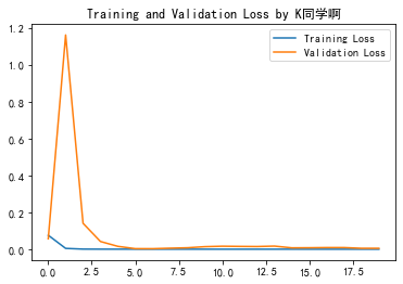
1. Draw loss Diagram
plt.plot(history.history['loss']    , label='Training Loss')
plt.plot(history.history['val_loss'], label='Validation Loss')
plt.title('Training and Validation Loss by K Classmates')
plt.legend()
plt.show()
2. Forecast
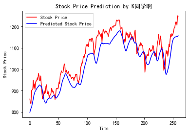
predicted_stock_price = model.predict(X_test)                        # Test Set Input Model for Prediction
predicted_stock_price = sc.inverse_transform(predicted_stock_price)  # Restore prediction data - from (0,1) de-normalization to original range
real_stock_price      = sc.inverse_transform(y_test)# Restore real data - from (0,1) de-normalization to original extent

# Draw a comparison curve between real and predicted data
plt.plot(real_stock_price, color='red', label='Stock Price')
plt.plot(predicted_stock_price, color='blue', label='Predicted Stock Price')
plt.title('Stock Price Prediction by K Classmates')
plt.xlabel('Time')
plt.ylabel('Stock Price')
plt.legend()
plt.show()
3. Assessment
"""
MSE  : mean square error    ----->  Predicted value minus true value squared and averaged
RMSE : Root mean square error  ----->  Square the mean square error
MAE  : Average Absolute Error----->  Predicted Value minus True Value Average after Absolute Value
R2   : The coefficient of determination can be simply understood as an important statistic reflecting the goodness of fit of the model

Detailed description can refer to the article: https://blog.csdn.net/qq_38251616/article/details/107997435
"""
MSE   = metrics.mean_squared_error(predicted_stock_price, real_stock_price)
RMSE  = metrics.mean_squared_error(predicted_stock_price, real_stock_price)**0.5
MAE   = metrics.mean_absolute_error(predicted_stock_price, real_stock_price)
R2    = metrics.r2_score(predicted_stock_price, real_stock_price)

print('mean square error: %.5f' % MSE)
print('Root mean square error: %.5f' % RMSE)
print('Average Absolute Error: %.5f' % MAE)
print('R2: %.5f' % R2)
mean square error: 2688.75170
 Root mean square error: 51.85317
 Average Absolute Error: 44.97829
R2: 0.74036
In addition to replacing the model, the fitness can be improved by adjusting the parameters. This paper mainly introduces LSTM, without detailing the adjustment of parameters.
Previous highlights:
- 100 Cases of in-depth Learning Convolutional Neural Network (CNN) for mnist Handwritten Number Recognition|Day 1
- Deep Learning 100 Cases-Convolution Neural Network (CNN) Clothing Image Classification|Day 3
- 100 in-depth learning - convolution neural network (CNN) flower recognition | Day 4
- In-depth Learning 100 Cases-Convolutional Neural Network (CNN) Weather Identification|Day 5
- Deep Learning 100 Cases-Convolutional Neural Network (VGG-16) Identify a gang of squid caps|Day 6
- Deep Learning 100 Cases-Convolutional Neural Network (ResNet-50) Bird Identification|Day 8
- In-depth Learning 100 Cases-Circulating Neural Network (RNN) Stock Forecasting|Day 9
From column: 100 Cases of Deep Learning
If you find this article helpful, remember to pay attention to it, give it a compliment, add a collection
Finally, I'll give you another copy to help you get the data structure refresh notes provided by first-line factories such as BAT, written by the big guys from Google and Arie, which are very useful for students who have weak algorithms or need to improve (Extraction Code: 9go2):
Leechtcode Titlebrush Notes for Google and Arie
And I've compiled 7K + open source e-books, there's always one that can help you 💖 (Extraction code: 4eg0)