Preface
I am following the monthly release of 2021.09.28: v2.17.0
This article explains the following:
- mmDetection Training Core Components
- mmDetection Test Core Components
- Build a faster rcnn configuration file using the core components above
There is no specific code implementation involved here, but familiarize yourself with the main components of the framework training and testing phases, as well as the interpretation of some parameters in the configuration file.
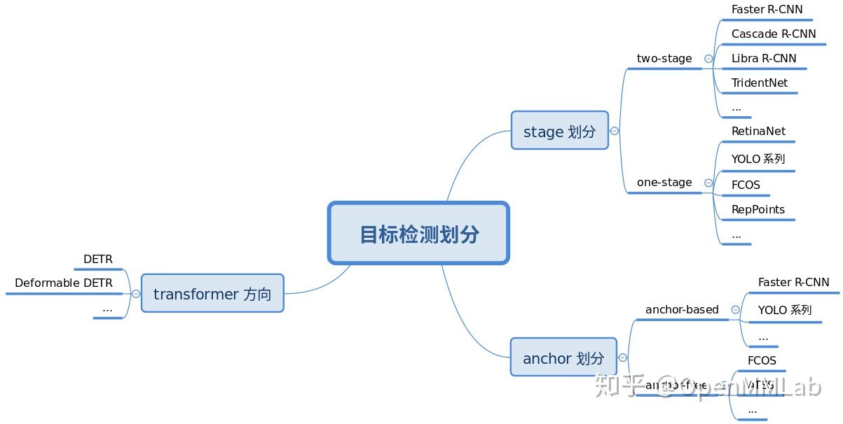
1. mmDetection Construction Process and Ideas
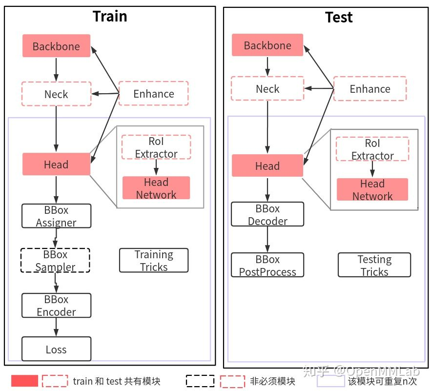
2. Training Core Components
The essential components are Backbone, Head, BBox Assign, BBox Encoder, Loss, Train Tricks.
Target Detection All Network Model Training Overall Process:
- Backbone: Any batch image is first entered into the backbone for feature extraction. A typical backbone has ResNet
- Neck: Input single-scale or multiscale feature map is input into neck module for feature fusion or enhancement, typical neck has FPN
- Head: Enter the fused or enhanced feature map into the head section for classification and regression prediction
- Enhance: Plug and Play enhancers can be introduced throughout the network building phase to enhance the network's feature extraction capabilities, such as SPP, DCN, and so on.
- Bbox Asssigner, Bbox Sampler: Target detection head er output is generally a feature map, for classification tasks there is a serious positive and negative sample imbalance, through positive and negative sample allocation and sampling control, balance positive and negative samples
- Bbox Encoder: gt bbox is typically encoded to facilitate convergence and balance of multiple branches
- Loss: The last step is to define classification and regression loss for training
- Train Tricks: There are many tricks included in the training process, such as optimizer selection, parameter tuning, etc.
2.1,Backbone
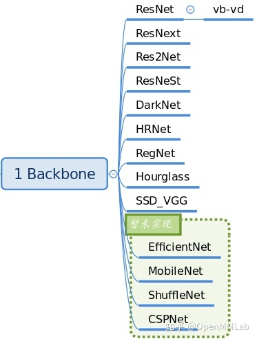
Backbones are primarily used for feature extraction and are stored in mmdet/models/backbones. The backbone network skeleton that has been implemented in the current version is as follows:
__all__ = [
    'RegNet', 'ResNet', 'ResNetV1d', 'ResNeXt', 'SSDVGG', 'HRNet',
    'MobileNetV2', 'Res2Net', 'HourglassNet', 'DetectoRS_ResNet',
    'DetectoRS_ResNeXt', 'Darknet', 'ResNeSt', 'TridentResNet', 'CSPDarknet',
    'SwinTransformer', 'PyramidVisionTransformer', 'PyramidVisionTransformerV2'
]
The ResNet family is most commonly used. If you need to extend Backbone, you can inherit the above network and register it for use through a registrar mechanism. A typical usage is in the configuration file:
    # The following are backbone configurations
    backbone=dict(
        # backbone type
        type='ResNet',
        # Network Layer Model Depth Use ResNet50
        depth=50,
        # Stage (Residual Module) Number of resnet Total including stem + 4 stage outputs
        num_stages=4,
        # The signature graph index (0, 1, 2, 3) representing the output of this module indicates that all four stage s output are fed into the subsequent fpn
        # Strides were (4,8,16,32) and channel s were (256,512,1024,2048) respectively.
        out_indices=(0, 1, 2, 3),
        # Which stage parameters are frozen i.e. the stage parameter is not trained
        frozen_stages=1,
        # Normalization layer Configuration Items Normalization layer categories are usually BN or GN where BN is used and the gamma and beta parameters in BN are trained
        norm_cfg=dict(type='BN', requires_grad=True),
        # The mean and variance of all BN layers of backbone are directly global pre-training values and are not updated
        norm_eval=True,
        # Network Code Style If pytorch is set, the layer stride 2 is conv3x3 convolution layer; If caffe is set, the layer stride 2 is the first conv1x1 convolution layer
        style='pytorch',
        # Use pytorch-provided weights trained on imagenet as pre-training weights
        init_cfg=dict(type='Pretrained', checkpoint='torchvision://resnet50')),
With the Registrar mechanism in MMCV, you can instantiate any registered class with dict configuration, which is very convenient and flexible.
2.2,Neck

Neck is responsible for efficiently fusing and enhancing backbone features, fusing input single- or multi-scale features, enhancing output, and so on. Store in: mmdet/model/necks file. The neck structure implemented in the current version is:
__all__ = [
    'FPN', 'BFP', 'ChannelMapper', 'HRFPN', 'NASFPN', 'FPN_CARAFE', 'PAFPN',
    'NASFCOS_FPN', 'RFP', 'YOLOV3Neck', 'FPG', 'DilatedEncoder',
    'CTResNetNeck', 'SSDNeck', 'YOLOXPAFPN'
]
The most common should be FPN, a typical use is in the configuration file:
    # The following are neck configurations
    neck=dict(
        # The neck type is FPN which also supports'NASFPN','PAFPN', etc.
        type='FPN',
        # The number of input channels corresponds to the number of output channels at each location of the backbone
        in_channels=[256, 512, 1024, 2048],
        # Number of output channels per neck layer
        out_channels=256,
        # Here an extra feature map is used to generate a larger proposal box using a higher feature map, i.e., num_in total Outs multi-scale feature maps
        num_outs=5),
2.3,Head
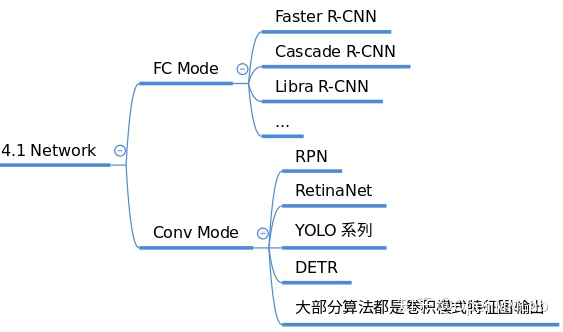
The output of target detection generally includes two branches, classification and frame coordinate regression. Different algorithms have different complexity and flexibility. In network construction, understanding the target detection algorithm is mainly to understand the head module. MMDetection stores ROI Heads divided into two-stage s in mmdet/models/roi_heads and one-stage enseHeads, stored in mmdet/models/dense_heads.
For example: dense_ Rpn_in heads Head:
    rpn_head=dict(
        # rpn_head type is RPNHead also supports'GARPNHead', etc.
        type='RPNHead',
        # The dimension of RPN input is dimension 256 of FPN output per layer above
        in_channels=256,
        # Number of channels for the first convolution layer
        feat_channels=256,
        # Configuration of anchor Generator produces anchors of different scales
        anchor_generator=dict(
            # Type is AnchorGenerator The anchor generator SSD used most is SSDAnchorGenerator
            type='AnchorGenerator',
            # Base ratio of anchor point, the area of anchor point at a location on the feature map is scale * base_sizes
            scales=[8],
            # anchor w h ratio
            ratios=[0.5, 1.0, 2.0],
            # Anchor generator step (down sampling rate) This is consistent with FPN characteristic step if base_is not set Sizes, the current step value will be treated as base_sizes
            strides=[4, 8, 16, 32, 64]),
        # Boxes need to be coded and decoded during training and testing
        bbox_coder=dict(
            # The category of the box encoder'DeltaXYWHBBoxCoder'is the most commonly used detail see: mmdet/core/bbox/coder/delta_xywh_bbox_coder.py
            type='DeltaXYWHBBoxCoder',
            # Mean value for encoding and decoding boxes
            target_means=[.0, .0, .0, .0],
            # Standard deviation for encoding and decoding boxes
            target_stds=[1.0, 1.0, 1.0, 1.0]),
        # Loss function configuration for classification branch of rpn subnetwork
        loss_cls=dict(
            # The use of cross-entropy loss also supports PN s such as FocalLoss, which are usually diclassified, so sigmoid functions are often used to classify branch loss weights=1
            type='CrossEntropyLoss', use_sigmoid=True, loss_weight=1.0),
        # Loss function configuration for regression branches of rpn subnetworks using L1Loss also supports IoU Losses and Smooth L1-loss as detailed below: mmdet/models/losses/smooth_l1_loss.py
        loss_bbox=dict(type='L1Loss', loss_weight=1.0)),
roi_heads:
roi_head=dict(
        # More details on the type of RoI head Reference: mmdet/models/roi_heads/standard_roi_head.py
        type='StandardRoIHead',
        # Step 1: Clip the feature map in the proposal box from the full feature map to output 256x7x7
        bbox_roi_extractor=dict(
            type='SingleRoIExtractor',
            # Using bilinear interpolation with the RoI-Align algorithm produces a 7x7 output regardless of the clipped proposal box.
            roi_layer=dict(type='RoIAlign', output_size=7, sampling_ratio=0),
            # Output channel unchanged or 256
            out_channels=256,
            # Specify how much of a pixel's displacement on a signature map corresponds to the original map
            featmap_strides=[4, 8, 16, 32]),
        # Step 2: Send a feature map of the same size clipped out to bbox head for classification + regression
        bbox_head=dict(
            # head of 2 Full Connection Layer Types
            type='Shared2FCBBoxHead',
            # Enter 256x7x7
            in_channels=256,
            # Change to 1024 through two full connection layer output channels
            fc_out_channels=1024,
            # Size of Region of Interest feature
            roi_feat_size=7,
            # Number of categories classified
            num_classes=80,
            # bbox encoder used in phase 2
            bbox_coder=dict(
                # Or use DeltaXYWHBBoxCoder as above rpn_head
                type='DeltaXYWHBBoxCoder',
                # Same as rpn_head
                target_means=[0., 0., 0., 0.],
                # Same as rpn_head
                target_stds=[0.1, 0.1, 0.2, 0.2]),
            # Is regression independent of category
            reg_class_agnostic=False,
            # Loss function configuration for classification branch of roi network is the same as rpn_above Head
            loss_cls=dict(
                type='CrossEntropyLoss', use_sigmoid=False, loss_weight=1.0),
            # Loss function configuration for classification branch of roi network is the same as rpn_above Head
            loss_bbox=dict(type='L1Loss', loss_weight=1.0))),
2.4,Enhance

enhance is a plug-and-play module that enhances features. Specific code can be easily registered as dict in backbone, neck, and head. Place in mmdet/models/
This part of the content is more cluttered, different enhance ment methods are called different methods, such as plugins in the ResNet skeleton, this part is not interpreted yet, read and explained in the specific algorithm module.
2.5,BBox Assigner
The function of the positive and negative sample attribute allocation module is to define positive and negative samples or assign positive and negative samples. Positive samples are background samples even if the foreground samples (can be any category). Because target detection is a problem of both classification and regression, classification scenarios need positive and negative samples to be trained. This module is critical because different positive and negative sample allocation strategies can result in significant performance differences. Some typical allocation strategies are as follows:
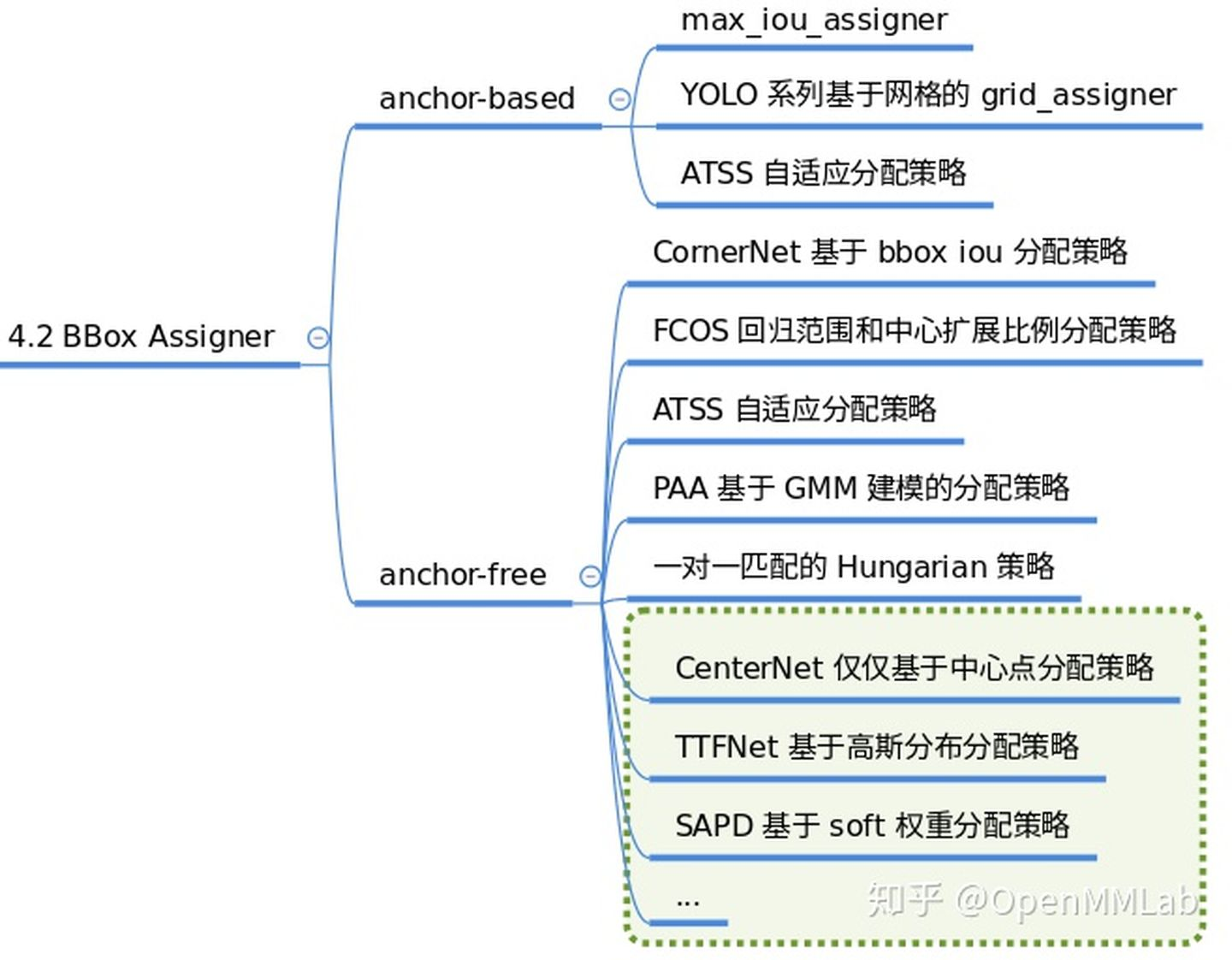
The corresponding code is placed in mmdet/core/bbox/assigners. The positive and negative sample matching strategies implemented by the current version are:
__all__ = [
    'BaseAssigner', 'MaxIoUAssigner', 'ApproxMaxIoUAssigner', 'AssignResult',
    'PointAssigner', 'ATSSAssigner', 'CenterRegionAssigner', 'GridAssigner',
    'HungarianAssigner', 'RegionAssigner', 'UniformAssigner', 'SimOTAAssigner'
]
A typical use is in a configuration file:
            assigner=dict(
                # Type of allocator MaxIoUAssigner iou-based allocation method used for many common detectors
                type='MaxIoUAssigner',
                # IoU >= 0.7 (threshold) is considered a positive sample
                pos_iou_thr=0.7,
                # IoU < 0.3 (threshold) is considered negative sample 0.3-0.7 regardless
                neg_iou_thr=0.3,
                # Use box as minimum IoU threshold for positive samples?
                min_pos_iou=0.3,
                # Whether to match low quality boxes (see API documentation for more details)
                match_low_quality=True,
                # Ignore the IoF threshold for bbox?
                ignore_iof_thr=-1),
2.6,BBox Sampler
After determining the positive and negative attributes of each sample, a sample balancing operation may be required. Because gt bbox is seldom used in target detection, the proportion of positive and negative samples is much smaller than 1. This often has one consequence: in the case of unbalanced datasets: for example, the number of negative samples is much larger than the number of positive samples, the whole training process is often manipulated by negative samples, and the loss function is also influenced by negative samples. To overcome this problem, an appropriate positive and negative sampling strategy is necessary. Typical sampling strategies are:
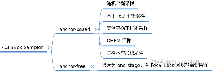
Corresponding code in: mmdet/core/bbox/samplers, positive and negative sampling strategies implemented by the current version are:
__all__ = [
    'BaseSampler', 'PseudoSampler', 'RandomSampler',
    'InstanceBalancedPosSampler', 'IoUBalancedNegSampler', 'CombinedSampler',
    'OHEMSampler', 'SamplingResult', 'ScoreHLRSampler'
]
A typical use is in a configuration file:
            sampler=dict(
                # Sampler type Use RandomSampler randomly here also supports PseudoSampler and other samplers to look at mmdet/core/bbox/samplers/
                type='RandomSampler',
                # Number of Samples
                num=256,
                # Proportion of positive samples to total samples
                pos_fraction=0.5,
                # Negative Sample Upper Limit Based on Positive Sample Number
                neg_pos_ub=-1,
                # Add GT as proposal after sampling
                add_gt_as_proposals=False),
2.7,BBox Encoder
In the regression part, it is often difficult to predict the xywh or xyxy coordinates of the direct prediction box, the size of coordinates is difficult to unify within a range, and it is difficult to predict the exact location for the network. So in order to better convergence and balance multiple loss es, we can use the bbox encoding strategy to use some kind of encoding transformation (inverse operation is bbox decoding) for gt bbox of positive samples. The simplest encoding strategy is to normalize the xy coordinates of gt bbox divided by the image width and log the wh to make better regression prediction. Some typical codec strategies are as follows:
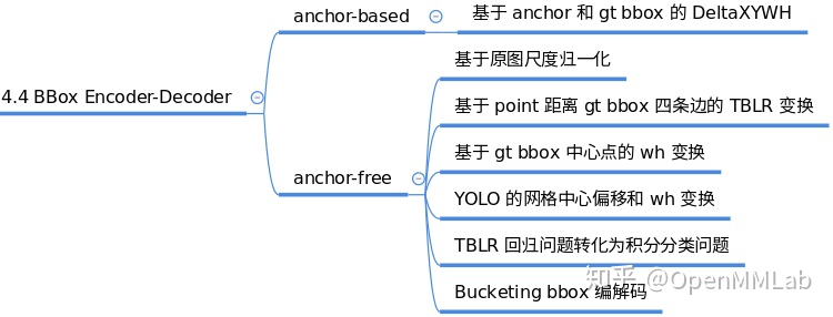
In mmdet/core/bbox/coder, the current version implements gt bbox codec strategies:
__all__ = [
    'BaseBBoxCoder', 'PseudoBBoxCoder', 'DeltaXYWHBBoxCoder',
    'LegacyDeltaXYWHBBoxCoder', 'TBLRBBoxCoder', 'YOLOBBoxCoder',
    'BucketingBBoxCoder'
]
A typical use is in a configuration file:
bbox_coder=dict(
                # Or use DeltaXYWHBBoxCoder as above rpn_head
                type='DeltaXYWHBBoxCoder',
                # Same as rpn_head
                target_means=[0., 0., 0., 0.],
                # Same as rpn_head
                target_stds=[0.1, 0.1, 0.2, 0.2]),
2.8,Loss
Loss modules are generally divided into classified loss and regression loss, which are iterative training for gradient descent of the predicted values from network head and the target values from bbox encoder. Loss design is also the focus of major algorithm improvements, commonly used loss as follows:
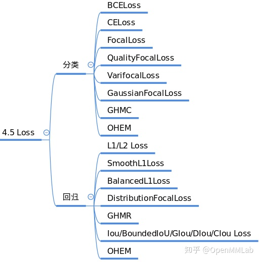
The corresponding code is in mmdet/models/losses, and the current version contains loss functions:
__all__ = [
    'accuracy', 'Accuracy', 'cross_entropy', 'binary_cross_entropy',
    'mask_cross_entropy', 'CrossEntropyLoss', 'sigmoid_focal_loss',
    'FocalLoss', 'smooth_l1_loss', 'SmoothL1Loss', 'balanced_l1_loss',
    'BalancedL1Loss', 'mse_loss', 'MSELoss', 'iou_loss', 'bounded_iou_loss',
    'IoULoss', 'BoundedIoULoss', 'GIoULoss', 'DIoULoss', 'CIoULoss', 'GHMC',
    'GHMR', 'reduce_loss', 'weight_reduce_loss', 'weighted_loss', 'L1Loss',
    'l1_loss', 'isr_p', 'carl_loss', 'AssociativeEmbeddingLoss',
    'GaussianFocalLoss', 'QualityFocalLoss', 'DistributionFocalLoss',
    'VarifocalLoss', 'KnowledgeDistillationKLDivLoss', 'SeesawLoss', 'DiceLoss'
]
A typical use is in a configuration file:
            # Loss function configuration for classification branch of roi network is the same as rpn_above Head
            loss_cls=dict(
                type='CrossEntropyLoss', use_sigmoid=False, loss_weight=1.0),
            # Loss function configuration for classification branch of roi network is the same as rpn_above Head
            loss_bbox=dict(type='L1Loss', loss_weight=1.0))),
2.9,Training trick
There are many training skills, and a large part of the work of adjusting parameters is to set this part of the super parameters. This part of the content is quite cluttered, and it is difficult to completely unify. The current mainstream tricks are as follows: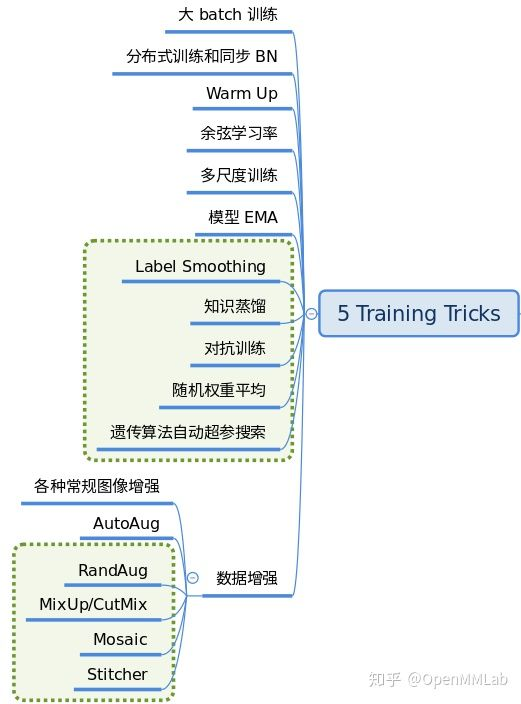
MMDetection is still improving this part.
3. Testing Core Components
Testing the core components is very similar to training, but it is much simpler. In addition to the necessary network building components (backbone, neck, head and enhance), there is no need for the three most difficult parts: positive and negative sample definition, positive and negative sample sampling, and loss calculation, but it requires an additional bbox postprocessing module and test trick.
3.1,BBox Decoder
gt bbox is coded during training and decoded during testing. Different encoding means different decoding. For example, when training, the encoding is to normalize xy divided by wh, and the corresponding decoding is multiplied by WH to get a prediction box relative to the original image. The code is also placed in the encoding folder, mmdet/core/bbox/coder.
3.2,BBox PostProcess
After the prediction box is obtained relative to the original image, the overlapping bbo phenomenon may occur, so post-processing is generally required. The common post-processing method is nms and its variants. The corresponding code is in mmdet/core/post_ In processing. Postprocessing methods implemented in the current version are:
__all__ = [
    'multiclass_nms', 'merge_aug_proposals', 'merge_aug_bboxes',
    'merge_aug_scores', 'merge_aug_masks', 'mask_matrix_nms', 'fast_nms'
]
3.3,Testing Tricks
trick is also used during the testing phase to improve test performance. There are many tricks in this stage, which are difficult to completely unify. The common testing strategies are as follows:
Insert a picture description here
The most typical are multiscale testing and various means of model integration, with typical configurations as follows:
dict(
    type='MultiScaleFlipAug',
    img_scale=(1333, 800),
    flip=True,
    transforms=[
        dict(type='Resize', keep_ratio=True),
        dict(type='RandomFlip'),
        dict(type='Normalize', **img_norm_cfg),
        dict(type='Pad', size_divisor=32),
        dict(type='ImageToTensor', keys=['img']),
        dict(type='Collect', keys=['img']),
    ])
4. Build Faster rcnn Model Profile
With the above components, we can easily set up a configuration file for the target detection framework, let's take faster rcnn for example.
# model settings
model = dict(
    # model Model Type
    type='FasterRCNN',
    # Backbone Configuration Information
    backbone=dict(
        # backbone type
        type='ResNet',
        # Network Layer Model Depth Use ResNet50
        depth=50,
        # Stage (Residual Module) Number of resnet Total including stem + 4 stage outputs
        num_stages=4,
        # The signature graph index (0, 1, 2, 3) representing the output of this module indicates that all four stage s output are fed into the subsequent fpn
        # Strides were (4,8,16,32) and channel s were (256,512,1024,2048) respectively.
        out_indices=(0, 1, 2, 3),
        # Which stage parameters are frozen i.e. the stage parameter is not trained
        frozen_stages=1,
        # Normalization layer Configuration Items Normalization layer categories are usually BN or GN where BN is used and the gamma and beta parameters in BN are trained
        norm_cfg=dict(type='BN', requires_grad=True),
        # The mean and variance of all BN layers of backbone are directly global pre-training values and are not updated
        norm_eval=True,
        # Network Code Style If pytorch is set, the layer stride 2 is conv3x3 convolution layer; If caffe is set, the layer stride 2 is the first conv1x1 convolution layer
        style='pytorch',
        # Use pytorch-provided weights trained on imagenet as pre-training weights
        init_cfg=dict(type='Pretrained', checkpoint='torchvision://resnet50')),
    # Neck Configuration Information
    neck=dict(
        # The neck type is FPN which also supports'NASFPN','PAFPN', etc.
        type='FPN',
        # The number of input channels corresponds to the number of output channels at each location of the backbone
        in_channels=[256, 512, 1024, 2048],
        # Number of output channels per neck layer
        out_channels=256,
        # Here an extra feature map is used to generate a larger proposal box using a higher feature map, i.e., num_in total Outs multi-scale feature maps
        # Enter the five-layer feature map generated by the FPN and generate a proposal box based on the five-layer feature map
        num_outs=5),
    # RPN_Head configuration information encapsulates the first step of a two-stage/cascade detector to extract candidate regions from the backbone generation signature map
    rpn_head=dict(
        # rpn_head type is RPNHead also supports'GARPNHead', etc.
        type='RPNHead',
        # The dimension of RPN input is dimension 256 of FPN output per layer above
        in_channels=256,
        # Number of channels for the first convolution layer
        feat_channels=256,
        # Configuration of anchor Generator produces anchors of different scales
        anchor_generator=dict(
            # Type is AnchorGenerator The anchor generator SSD used most is SSDAnchorGenerator
            type='AnchorGenerator',
            # Base ratio of anchor point, the area of anchor point at a location on the feature map is scale * base_sizes
            scales=[8],
            # anchor w h ratio
            ratios=[0.5, 1.0, 2.0],
            # Anchor generator step (down sampling rate) This is consistent with FPN characteristic step if base_is not set Sizes, the current step value will be treated as base_sizes
            strides=[4, 8, 16, 32, 64]),
        # Boxes need to be coded and decoded during training and testing
        bbox_coder=dict(
            # The category of the box encoder'DeltaXYWHBBoxCoder'is the most commonly used detail see: mmdet/core/bbox/coder/delta_xywh_bbox_coder.py
            type='DeltaXYWHBBoxCoder',
            # Mean value for encoding and decoding boxes
            target_means=[.0, .0, .0, .0],
            # Standard deviation for encoding and decoding boxes
            target_stds=[1.0, 1.0, 1.0, 1.0]),
        # Loss function configuration for classification branch of rpn subnetwork
        loss_cls=dict(
            # The use of cross-entropy loss also supports PN s such as FocalLoss, which are usually diclassified, so sigmoid functions are often used to classify branch loss weights=1
            type='CrossEntropyLoss', use_sigmoid=True, loss_weight=1.0),
        # Loss function configuration for regression branches of rpn subnetworks using L1Loss also supports IoU Losses and Smooth L1-loss as detailed below: mmdet/models/losses/smooth_l1_loss.py
        loss_bbox=dict(type='L1Loss', loss_weight=1.0)),
    # ROI-Head configuration information RoIHead encapsulates the second step of a two-stage/cascade detector
    # ROI-Head predicts population in two-step bbox_based on the feature map of the proposal box and original map produced by RPN-Head Roi_ Extractor + bbox_ Head
    roi_head=dict(
        # More details on the type of RoI head Reference: mmdet/models/roi_heads/standard_roi_head.py
        type='StandardRoIHead',
        # Step 1: Clip the feature map in the proposal box from the full feature map to output 256x7x7
        bbox_roi_extractor=dict(
            type='SingleRoIExtractor',
            # Using bilinear interpolation with the RoI-Align algorithm produces a 7x7 output regardless of the clipped proposal box.
            roi_layer=dict(type='RoIAlign', output_size=7, sampling_ratio=0),
            # Output channel unchanged or 256
            out_channels=256,
            # Specify how much of a pixel's displacement on a signature map corresponds to the original map
            featmap_strides=[4, 8, 16, 32]),
        # Step 2: Send a feature map of the same size clipped out to bbox head for classification + regression
        bbox_head=dict(
            # head of 2 Full Connection Layer Types
            type='Shared2FCBBoxHead',
            # Enter 256x7x7
            in_channels=256,
            # Change to 1024 through two full connection layer output channels
            fc_out_channels=1024,
            # Size of Region of Interest feature
            roi_feat_size=7,
            # Number of categories classified
            num_classes=80,
            # bbox encoder used in phase 2
            bbox_coder=dict(
                # Or use DeltaXYWHBBoxCoder as above rpn_head
                type='DeltaXYWHBBoxCoder',
                # Same as rpn_head
                target_means=[0., 0., 0., 0.],
                # Same as rpn_head
                target_stds=[0.1, 0.1, 0.2, 0.2]),
            # Is regression independent of category
            reg_class_agnostic=False,
            # Loss function configuration for classification branch of roi network is the same as rpn_above Head
            loss_cls=dict(
                type='CrossEntropyLoss', use_sigmoid=False, loss_weight=1.0),
            # Loss function configuration for classification branch of roi network is the same as rpn_above Head
            loss_bbox=dict(type='L1Loss', loss_weight=1.0))),
    # model training and testing settings sampling training configuration testing nms configuration
    # Configuring the behavior of some modules during training
    train_cfg=dict(
        # rpn module training behavior configuration
        rpn=dict(
            # 1. When assigning positive and negative sample training in the first stage, you need to compare the gt box with the proposal box (anchor) generated by the RPN to classify and return the target values of the proposal box
            assigner=dict(
                # Type of allocator MaxIoUAssigner iou-based allocation method used for many common detectors
                type='MaxIoUAssigner',
                # IoU >= 0.7 (threshold) is considered a positive sample
                pos_iou_thr=0.7,
                # IoU < 0.3 (threshold) is considered negative sample 0.3-0.7 regardless
                neg_iou_thr=0.3,
                # Use box as minimum IoU threshold for positive samples?
                min_pos_iou=0.3,
                # Whether to match low quality boxes (see API documentation for more details)
                match_low_quality=True,
                # Ignore the IoF threshold for bbox?
                ignore_iof_thr=-1),
            # 2. Phase 1 Positive and Negative Sample Sampling From rpn Assigned thousands of Positive and Negative Sample Proposal Boxes but not all of them will participate in training but 256 randomly sampled Proposal Boxes for training
            sampler=dict(
                # Sampler type Use RandomSampler randomly here also supports PseudoSampler and other samplers to look at mmdet/core/bbox/samplers/
                type='RandomSampler',
                # Number of Samples
                num=256,
                # Proportion of positive samples to total samples
                pos_fraction=0.5,
                # Negative Sample Upper Limit Based on Positive Sample Number
                neg_pos_ub=-1,
                # Add GT as proposal after sampling
                add_gt_as_proposals=False),
            # Borders allowed after filling valid anchors?
            allowed_border=-1,
            # Weight of positive samples during training
            pos_weight=-1,
            # Whether to set debug mode
            debug=False),
        # rpn generates candidate box behavior configuration: 2000 candidate boxes from rpn training 1000 candidate boxes from nms and 256 from 1000 for training
        rpn_proposal=dict(
            # Number of box es before NMS
            nms_pre=2000,
            # Maximum number of box es to keep after NMS
            max_per_img=1000,
            # nms Configuration nms Category=Threshold of iou in nms NMS
            nms=dict(type='nms', iou_threshold=0.7),
            # Minimum box size allowed
            min_bbox_size=0),
        # rcnn module training behavior configuration
        rcnn=dict(
            # 1. Stage 2 Assignment Positive and Negative Sample Configuration Interpretation Same as above
            assigner=dict(
                type='MaxIoUAssigner',
                pos_iou_thr=0.5,
                neg_iou_thr=0.5,
                min_pos_iou=0.5,
                match_low_quality=False,
                ignore_iof_thr=-1),
            # 2. Interpretation of positive and negative sample configurations for the second stage of sampling as above
            sampler=dict(
                type='RandomSampler',
                num=512,
                pos_fraction=0.25,
                neg_pos_ub=-1,
                add_gt_as_proposals=True),
            pos_weight=-1,
            debug=False)),
    # Some parameters in the testing phase control the testing behavior configuration as explained above
    test_cfg=dict(
        rpn=dict(
            nms_pre=1000,
            max_per_img=1000,
            nms=dict(type='nms', iou_threshold=0.7),
            min_bbox_size=0),
        rcnn=dict(
            score_thr=0.05,
            nms=dict(type='nms', iou_threshold=0.5),
            max_per_img=100)
        # soft-nms is also supported for rcnn testing
        # e.g., nms=dict(type='soft_nms', iou_threshold=0.5, min_score=0.05)
    ))
Reference
Official Documents.
Official Knowledge Interpretation.
Interpretation of Official b Station: [OpenMMLab Subtitle Version of General Visual Frame] Lecture 4 Target Detection & MMDetection (2)-Dr. Chen Kai.