Running environment and compiling tools
- Windows
- VS Code
Programming language and library version
| library | edition |
|---|---|
| Python | 3.7.0 |
| copy | nothing |
| numpy | 1.19.2 |
| opencv | 3.4.2 |
| PIL | 8.1.0 |
| matplotlib | 3.4.3 |
Question 1 black and white image grayscale scanning (20 points)
Implement a function s = scanLine4e(f, I, loc), where f is a gray image, I is an integer, and loc is a string. When loc is' row ', I represents the number of rows. When loc is' column ', I represents the number of columns. The output s is the pixel gray value vector of the corresponding related row or column.
Procedure:
# Call Toolkit
import numpy as np
import cv2
from PIL import Image
import matplotlib.pyplot as plt
def scanLine4e(f,I,loc):
    try:
        # Judge the type of I. when the row / column is even, I is of list type and returns the average value of pixels in the middle two rows
        if type(I) is int:
            if loc == "row":
                s = f[I,:]
            elif loc == "column":
                s = f[:,I]
        else:
            if loc == "row":
                s = np.sum(f[I[0]:I[1]+1,:],axis=0) / 2
                s = np.int16(s)
            elif loc == "column":
                s = np.sum(f[:,I[0]:I[1]+1],axis=1) / 2
                s = np.int16(s)

        print(s)
        return s
    except:
        print("Please enter the correct parameter value")
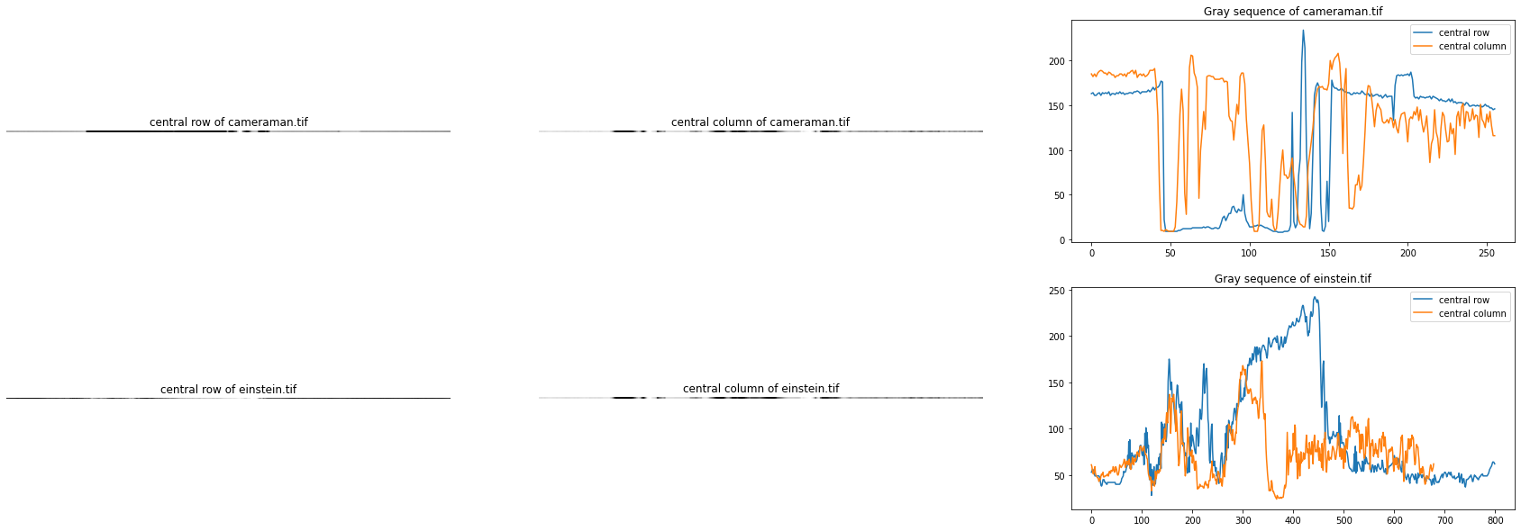
Call this function to extract the pixel gray vector of the central row and column of cameraman.tif and einstein.tif, and draw the scanned gray sequence into a graph.
function:
# Get the center of the image. When the width or length of the image is an even number, take the middle two rows / columns and store them as a list array. When it is an odd number, they are stored as int
def get_center(L):
    if L % 2 == 0:
        I = [int(H1 / 2) - 1,int(H1 / 2)]
    else:
        I = int(H1 / 2)
    return I

cameraman = np.array(Image.open('./cameraman.tif'))
H1,W1 = cameraman.shape
print("cameraman.tif The size of the is({},{})".format(H1,W1))
I1_row = get_center(H1)
s1_row = scanLine4e(cameraman,I1_row,"row")
s1_row = s1_row.reshape(1,W1)
I1_column = get_center(W1)
s1_column = scanLine4e(cameraman,I1_column,"column")
s1_column = s1_column.reshape(1,H1)

einstein = np.array(Image.open('./einstein.tif'))
H2,W2 = einstein.shape
print("einstein.tif The size of the is({},{})".format(H2,W2))
I2_row = get_center(H2)
s2_row = scanLine4e(einstein,I2_row,"row")
s2_row = s2_row.reshape(1,W2)
I2_column = get_center(W2)
s2_column = scanLine4e(einstein,I2_column,"column")
s2_column = s2_column.reshape(1,H2)

plt.figure(figsize=(30,10))
plt.subplot(2,3,1)
plt.title("central row of cameraman.tif")
plt.axis('off')
plt.imshow(s1_row,cmap='gray')

plt.subplot(2,3,2)
plt.title("central column of cameraman.tif")
plt.axis('off')
plt.imshow(s1_column,cmap='gray')

plt.subplot(2,3,3)
plt.title("Gray sequence of cameraman.tif")
plt.plot(s1_row[0,:],label = 'central row')
plt.plot(s1_column[0,:],label = 'central column')
plt.legend()

plt.subplot(2,3,4)
plt.title("central row of einstein.tif")
plt.axis('off')
plt.imshow(s2_row,cmap = 'gray')

plt.subplot(2,3,5)
plt.title("central column of einstein.tif")
plt.axis('off')
plt.imshow(s1_column,cmap = 'gray')

plt.subplot(2,3,6)
plt.title("Gray sequence of einstein.tif")
plt.plot(s2_row[0,:],label = 'central row')
plt.plot(s2_column[0,:],label = 'central column')
plt.legend()
plt.savefig("Q1.png")
plt.show()
Output:
cameraman.tif The size of the is(256,256)
[163 164 161 161 163 164 161 164 163 164 163 165 161 163 163 162 164 163
 165 163 164 162 163 163 164 164 163 165 165 166 165 163 165 165 165 165
 167 165 167 170 167 170 170 172 177 176  22   9   9   9   9   9   9   9
   9  10  10  11  12  12  12  12  12  12  13  13  13  13  13  13  13  14
  13  14  14  13  12  12  13  13  12  13  18  24  26  21  25  29  29  36
  37  32  30  34  32  32  50  29  21  18  14  14  14  15  15  16  15  16
  15  14  13  13  12  11  10   9   9   9   8   8   8   8   9   9   9  10
  16 142  20  13  17  71  90 198 234 214  98  60  12  29  93 161 171 175
 170  41  10   9  15  65  20  99 178 171 169 169 167 167 169 167 165 165
 164 164 162 162 164 163 164 163 163 166 164 162 162 163 160 163 160 161
 162 162 160 161 158 160 162 159 160 160 160 133 172 183 184 183 184 183
 184 184 185 183 187 179 160 158 159 157 160 159 159 158 159 159 160 157
 160 159 158 157 155 157 155 155 154 155 157 154 157 153 154 152 153 153
 153 152 150 153 152 149 149 150 150 149 150 149 150 148 149 151 149 149
 147 147 145 146]
[185 182 185 182 186 188 189 188 186 186 184 187 186 184 184 181 183 183
 185 185 183 185 182 186 186 188 189 185 189 181 184 185 183 185 182 183
 Limited space, only part of the exhibition...
Question 2: convert color image to black-and-white image (20 points)
A common problem in image processing is to convert color RGB image into monochrome gray image. The first common method is to take the mean value of three elements R, G and B. The second common method, also known as NTSC standard, takes into account human color perception experience. Different weighting coefficients are adopted for R, G and B channels, namely R channel 0.2989, G channel 0.5870 and B channel 0.1140. A function g = rgb1gray(f, method) is realized. The function function is to convert a 24 bit RGB image, f, into a gray image, g. Parameter method is a string. When its value is' average ', the first conversion method is adopted. When its value is' NTSC', the second conversion method is adopted. Use 'NTSC' as the default.
Procedure:
def rgb1gray(f, method = "average"):
    R = f[:,:,0]
    G = f[:,:,1]
    B = f[:,:,2]
    try:
        if method == "average":
            # Note that the title says a 32-bit image
            g = np.int32((R + G + B) / 3)
        elif method == "NTSC":
            g = np.int32(0.2989*R + 0.5870*G + 0.1140*B)
        return g
    except:
        print("Parameter error")
Call this function to mandril the provided image_ Color.tif and lena512color.tiff are converted into monochrome gray images by the above two methods. The results of the two methods are briefly compared and discussed.
function:
img1 = Image.open("./mandril_color.tif")
img1 = np.array(img1)
g1_average = rgb1gray(img1,"average")
g1_NTSC = rgb1gray(img1,"NTSC")


img2 = Image.open("./lena512color.tiff")
img2 = np.array(img2)
g2_average = rgb1gray(img2,"average")
g2_NTSC = rgb1gray(img2,"NTSC")

plt.figure(figsize=(10,10))
plt.subplot(2,2,1)
plt.title("mandril_color average gray")
plt.imshow(g1_average,cmap='gray')

plt.subplot(2,2,2)
plt.title("mandril_color NTSC gray")
plt.imshow(g1_NTSC,cmap='gray')

plt.subplot(2,2,3)
plt.title("lena512color average gray")
plt.imshow(g2_average,cmap='gray')

plt.subplot(2,2,4)
plt.title("lena512color NTSC gray")
plt.imshow(g2_NTSC,cmap='gray')
plt.show()
Output:
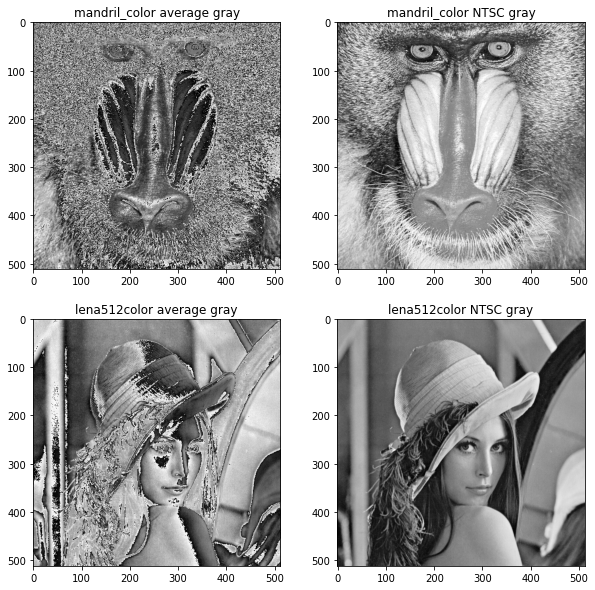
Discuss the differences between the two gray images
As can be seen from the results NTSC The grayscale image generated by the format looks more comfortable, smooth and delicate. At first I didn't know why. After consulting the data
NTCS Considering the different degree of light perception of human eyes. There are several cone-shaped photoreceptor cells in human eyes, which are most sensitive to yellow green, green and blue purple light. Although the vertebral cells in the eyeball do not have the strongest sensitivity to the three colors of red, green and blue, the bandwidth of light that can be felt by the vertebral cells of the naked eye is large, and red, green and blue can also stimulate the light receptors of these three colors independently.
The order of human perception of red, green and blue is green>red>Blue, so the average algorithm is unscientific from this point of view. A weight should be set for each color according to the degree of human perception of light, and their status should not be equal.
Question 3 image two-dimensional convolution function (20 points)
Implement a function g = twodConv(f, w), where f is a gray source image and W is a rectangular convolution kernel. The output image G is required to be consistent with the size of the source image f (that is, the number of rows and columns of pixels). Note that to meet this requirement, boundary pixel padding is required for the source image F. Here, please implement two schemes. The first scheme is pixel copy. The corresponding option is defined as' replicate ', and the filled pixel copy is grayscale with its nearest image boundary pixel. The second scheme is to fill zero. The corresponding option is defined as' zero ', and the filled pixel gray is 0. Set the second scheme as the default choice.
Procedure:
def twoConv(f,w,method = "replicate"):
    # The width the image should extend
    pad_width = w.shape[0] - 1
    # Convolution kernel size
    w_size = w.shape[0]
    pad_width_one = int(pad_width / 2)
    H,W = f.shape
    # Zero space of image size after creating padding
    img_pad = np.zeros([H+pad_width,W+pad_width],dtype=np.int16)
    # Fill the pixels of the original image, and the padding operation is performed in the extended part
    img_pad[pad_width_one:H+pad_width_one,pad_width_one:W+pad_width_one] = f
    if method == "replicate":
        for i in range(pad_width_one):
            # Fill four edges and four corners respectively
            img_pad[i:i+1,pad_width_one:W+pad_width_one] = f[0,:]
            img_pad[H+pad_width_one+i:H+pad_width_one+i+1,pad_width_one:W+pad_width_one] = f[-1,:]
            img_pad[pad_width_one:H+pad_width_one,i:i+1] = f[:,0].reshape([H,1])
            img_pad[pad_width_one:H+pad_width_one,W+pad_width_one+i:W+pad_width_one+i+1] = f[:,-1].reshape([H,1])
        img_pad[0:pad_width_one,0:pad_width_one] = f[0,0] * np.ones([pad_width_one,pad_width_one])
        img_pad[0:pad_width_one,W+pad_width_one:W+2*pad_width_one] = f[0,-1] * np.ones([pad_width_one,pad_width_one])
        img_pad[H+pad_width_one:H+2*pad_width_one,0:pad_width_one] = f[-1,0] * np.ones([pad_width_one,pad_width_one])
        img_pad[H+pad_width_one:H+2*pad_width_one,W+pad_width_one:W+2*pad_width_one] = f[-1,-1] * np.ones([pad_width_one,pad_width_one])
    elif method == "zero":
        pass
    g = np.zeros([H,W],dtype=np.int16)
    flatten_w = w.reshape([1,w_size**2])
    # The process of convolution is flattened first, and the inner product of column and row vectors is carried out
    for i in range(H):
        for j in range(W):
            g[i,j] = np.dot(flatten_w,img_pad[i:w_size+i,j:w_size+j].reshape([w_size**2,1]))
    return g
Question 4 normalized two-dimensional Gaussian filtering kernel function (20 points)
Implement a Gaussian filtering kernel function w = gaussKernel(sig, m), where sig corresponds to the value in the definition of Gaussian function σ, The size of W is m × m. Please note that if M is not provided here, it needs to be calculated and determined. If M has been provided but is too small, a warning message shall be given. W requires normalization, that is, the sum of all elements is 1.
def gaussKernel(sig,*m):
    # Provided by convolution kernel to judge whether the size is appropriate m > = 6 * sig + 1
    if m:
        l = m[0]
        if l < (6*sig + 1) or l%2 == 0:
            print("Convolution kernel size is too small or even, please re-enter!")
            return 0
    else:
        l = int(6*sig + 1)
        if l%2 ==0:
            l += 1
    w = np.zeros([1,l],dtype=np.float32)
    for i in range(l):
        # w[0,i] = pow(pow(2*np.pi,0.5)*sig,-1)*pow(np.e,-pow((i-int((l-1)/2))/((2**0.5)*sig),2))
        # Due to normalization, the coefficient of normal distribution about pi is rounded off, which does not affect the result
        w[0,i] = pow(sig,-1)*pow(np.e,-pow((i-int((l-1)/2))/((2**0.5)*sig),2))
    w = np.dot(w.T,w)
    w = w / np.sum(w)
    return w
Question 5 Gaussian filtering of gray image (20 points)
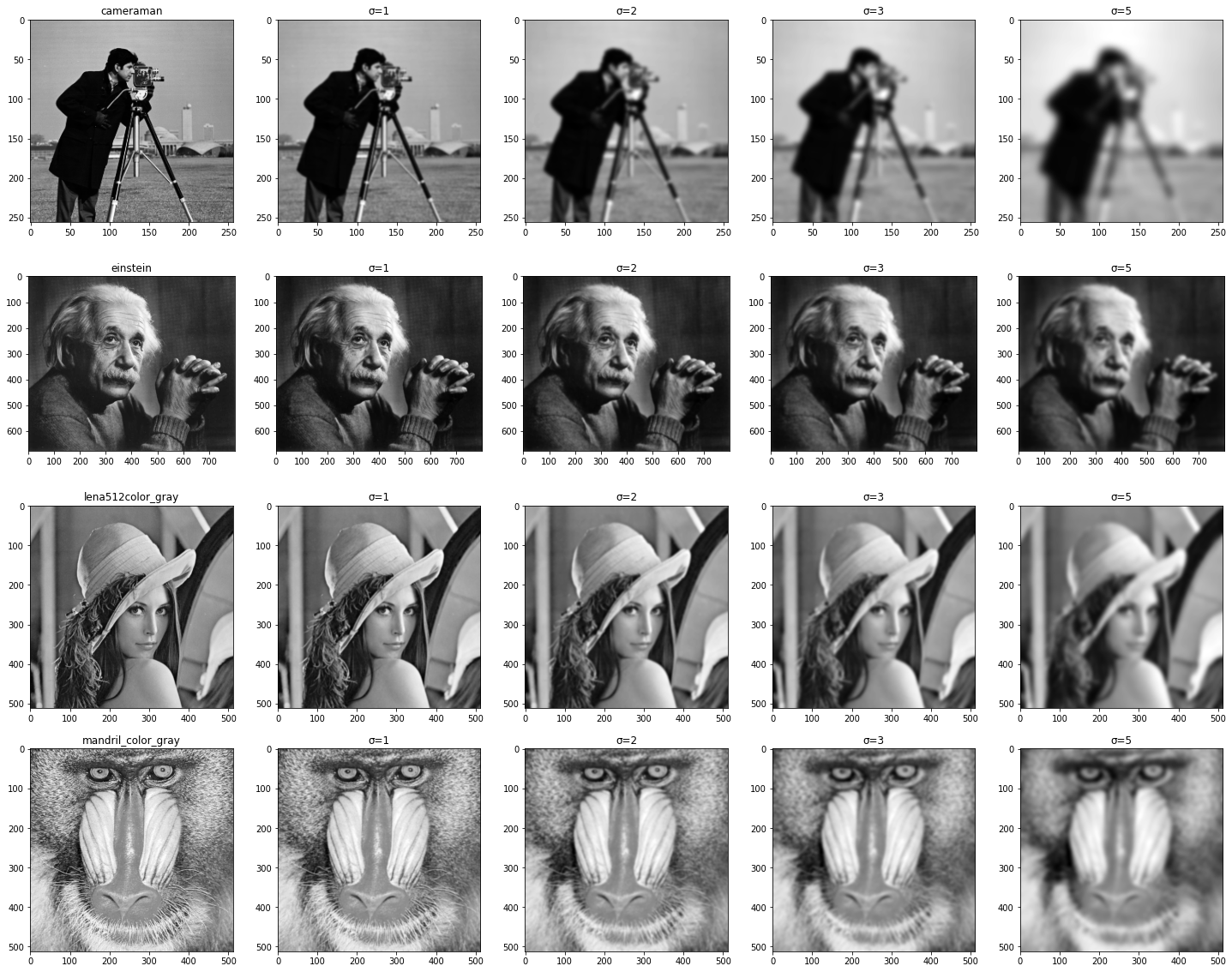
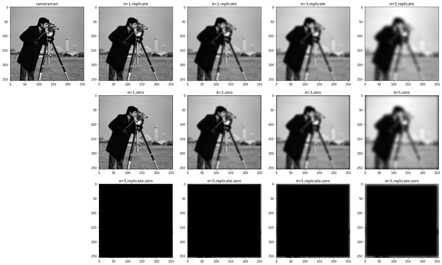
Call the function implemented above to perform Gaussian filtering on the gray images (cameraman, einstein, and NTSC converted gray images corresponding to lena512color and mandril_color) in questions 1 and 2 σ= 1,2,3,5. Select any pixel filling scheme. about σ= The results under 1 are compared with the results of directly calling the relevant functions of MATLAB or Python software package (the difference image can be simply calculated). Then, select any two images and compare the difference between pixel copy and subzero filtering results on the boundary when other parameters are unchanged.
use σ= 1, 2, 3, 5. The pixel filling scheme is replicate
cameraman = np.array(Image.open('cameraman.tif'))
einstein = np.array(Image.open('einstein.tif'))
lena512color = np.array(Image.open('lena512color.tiff'))
lena512color_gray = rgb1gray(lena512color,method='NTSC')
mandril_color = np.array(Image.open('mandril_color.tif'))
mandril_color_gray = rgb1gray(mandril_color,method='NTSC')
plt.figure(figsize=(25,20))
imgs = [cameraman,einstein,lena512color_gray,mandril_color_gray]
img_names = ["cameraman","einstein","lena512color_gray","mandril_color_gray"]
sigs = [1,2,3,5]
num = 1
for img in imgs:
    plt.subplot(4,5,num)
    plt.title('{}'.format(img_names[num // 5]))
    plt.imshow(img,cmap='gray')
    num += 1
    for sig in sigs:
        w = gaussKernel(sig)
        g = twoConv(img,w)
        plt.subplot(4,5,num)
        plt.title('σ={}'.format(sig))
        plt.imshow(g,cmap='gray')
        num += 1
plt.show()
about σ= 1, directly call Python opencv(3.4.2) for comparison (you can simply calculate the difference image)
plt.figure(figsize=(30,20))
num = 1
w = gaussKernel(1)
for img in imgs:
    img_pxels = img.size
    plt.subplot(4,6,num)
    plt.title('{}'.format(img_names[num // 6]))
    plt.imshow(img,cmap='gray')

    # opencv
    num += 1
    im_cv = cv2.GaussianBlur(np.int16(img), (7, 7),1,1)
    plt.subplot(4,6,num)
    plt.title('OpenCV')
    plt.imshow(im_cv,cmap='gray')

    # My method
    num += 1
    g = twoConv(img,w)
    plt.subplot(4,6,num)
    plt.title('My method')
    plt.imshow(g,cmap='gray')

    #  Pixel difference  == 0  0,or 255
    num += 1
    #  Mask: 0 when the pixel values are equal, and black in the image; If the pixels are different, it is 255 and white in the image, the same below
    mask = np.where(g == im_cv,0,255)
    mask_pxels = np.sum(mask == 0)
    plt.subplot(4,6,num)
    plt.title('Pixel difference==0 ratio:{:.3f}'.format(mask_pxels/img_pxels))
    plt.imshow(mask,cmap='gray')

    #  Pixel difference  <= 1  0,or 255
    num += 1
    mask = np.where(np.abs(g - im_cv) <= 1,0,255)
    mask_pxels = np.sum(mask == 0)
    plt.subplot(4,6,num)
    plt.title('Pixel difference<=1 ratio:{:.3f}'.format(mask_pxels/img_pxels))
    plt.imshow(mask,cmap='gray')

    #  Pixel difference  <= 2  0,or 255
    num += 1
    mask = np.where(np.abs(g - im_cv) <= 2,0,255)
    mask_pxels = np.sum(mask == 0)

    plt.subplot(4,6,num)
    plt.title('Pixel difference<=2 ratio:{:.3f}'.format(mask_pxels/img_pxels))
    plt.imshow(mask,cmap='gray')
    num += 1
plt.show()
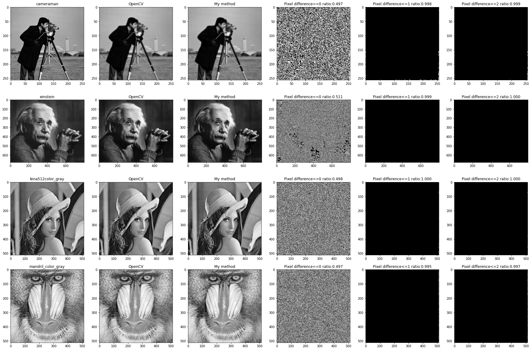
You can see that the Gaussian convolution program written by yourself is similar to OpenCV Compared with the built-in convolution, the exact proportion of pixels is about 50%,And the distribution is scattered, and there is no obvious law.
However, when the allowable pixel difference is within 1, the similarity reaches 99%above; When the tolerance is within 2, the two methods are basically the same. Different places are mainly concentrated in the boundary area.
cameraman.tif and einstein.tif are selected to compare the difference of pixel replication and subzero filtering results on the boundary when other parameters are unchanged
cameraman.tif
# If you change imgs, you can select different images, and the other programs are the same
imgs = [cameraman]
plt.figure(figsize=(25,15))
sigs = [1,2,3,5]
num = 1
replicate = []
zero = []
for img in imgs:
    plt.subplot(3,5,num)
    plt.title('{}'.format('cameraman'))
    plt.imshow(img,cmap='gray')
    num += 1
    for sig in sigs:
        w = gaussKernel(sig)
        g = twoConv(img,w)
        replicate.append(g)
        plt.subplot(3,5,num)
        plt.title('σ={},replicate'.format(sig))
        plt.imshow(g,cmap='gray')
        num += 1
    num += 1
    for sig in sigs:
        w = gaussKernel(sig)
        g = twoConv(img,w,method='zero')
        zero.append(g)
        plt.subplot(3,5,num)
        plt.title('σ={},zero'.format(sig))
        plt.imshow(g,cmap='gray')
        num += 1
    num += 1
    for i in range(len(sigs)):
        mask = replicate[i] - zero[i]
        plt.subplot(3,5,num)
        plt.title('σ={},replicate-zero'.format(sig))
        plt.imshow(mask,cmap='gray')
        num += 1

plt.show()
einstein.tif
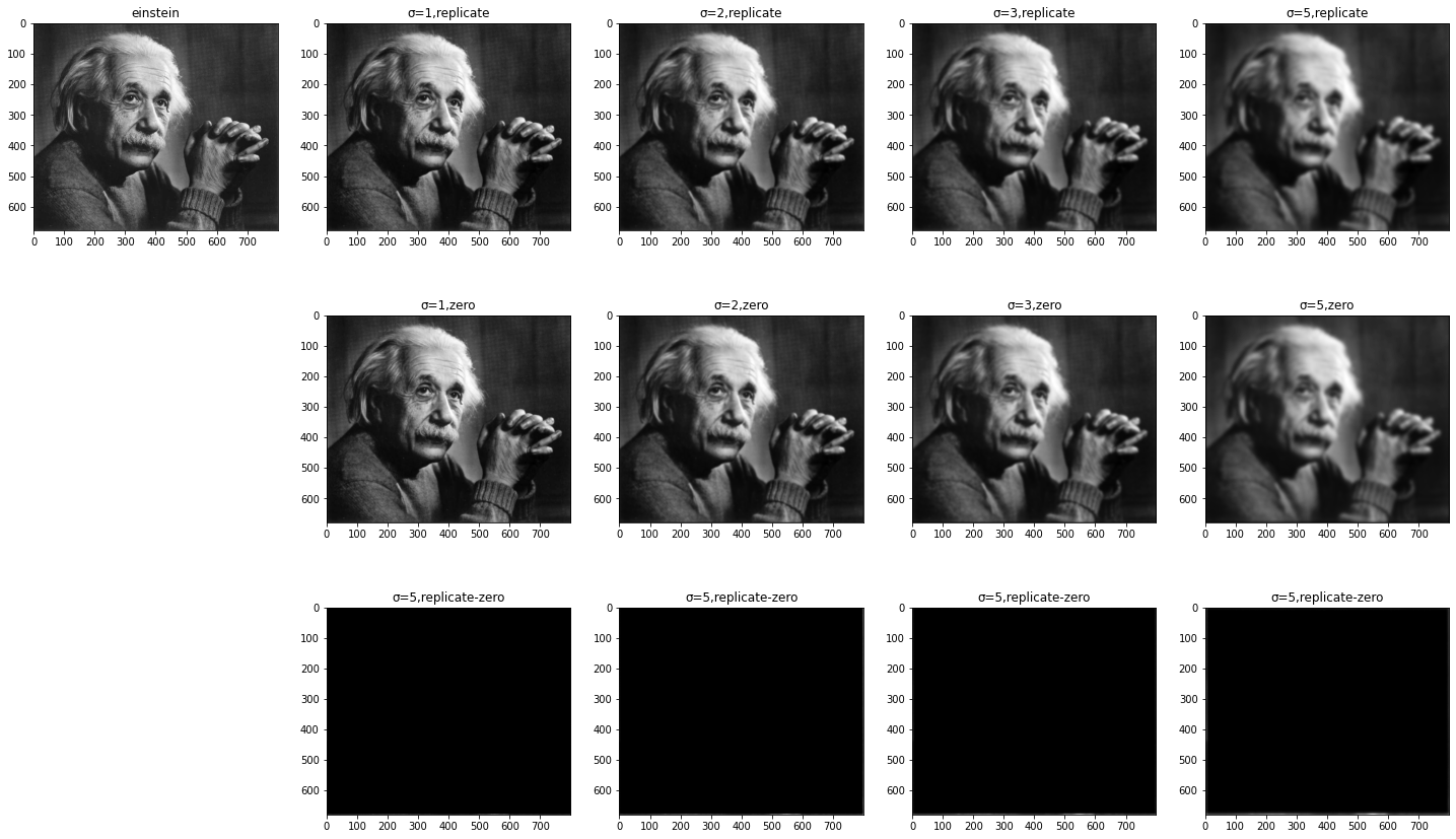
It can be seen that when the filling method is to copy the nearest pixel, the result after convolution is better, and zero The boundary of the two methods will become dark after zero filling, and the difference between the two methods mask It's also reflected, replicate Image boundary ratio after convolution zero The boundary of the mode is bright
#### @Time    : 2021/10/8 10:49
#### @Author  : AlanLiang
#### @FileName: HW_1.ipynb
#### @Software: VS Code
#### @Github  : https://github.com/AlanLiangC
#### @Mail    : liangao21@mails.ucas.ac.cn