Machine learning -- logistic regression (multivariate classification) programming training
reference material:
1.Mr. Huang haiguang: Wu Enda machine learning notes github
This paper is the first part of the third programming training in Wu Enda's machine learning course.
Programming tasks:
Recognize handwritten digits (0 to 9) using logical regression
Dataset: GitHub warehouse from Mr. Huang haiguang, Specific links

This dataset is a. mat file containing two variables X , y X,y X,y
variable X X X ¢ sample pictures containing 5000 handwritten digits, each sample picture is 20 in size × 20 pixels, so each sample is represented as 400 dimensions, where the value represents the gray value of each pixel lattice.
variable y y y is the label corresponding to 5000 samples, such as 1-500 samples y = 10 y = 10 y=10, indicating that the 500 samples are corresponding to class 0, 501-1000 samples y = 1 y = 1 y=1, indicating that the 500 samples correspond to class 1. If this goes on, y y The value of y ranges from 1-10, corresponding to numbers 1-9 and 0 respectively
1. Multivariate classification
adopt Machine learning -- logistic regression (classification) programming training We are already familiar with the binary classification problem.
The so-called multivariate classification can be understood as: the reclassification of secondary classification.
For example, we want to classify dataset a into four categories: A, B, C and d. First, we can divide a into a and B, then B into B and C, and finally C into C and d.
This multiple classification problem is based on two classification, which can be called one vs others classification.
Multivariate classification problem is actually realized by using multiple binary classifiers, which is essentially the same as logistic regression binary classification problem.
2. Label Vectorization
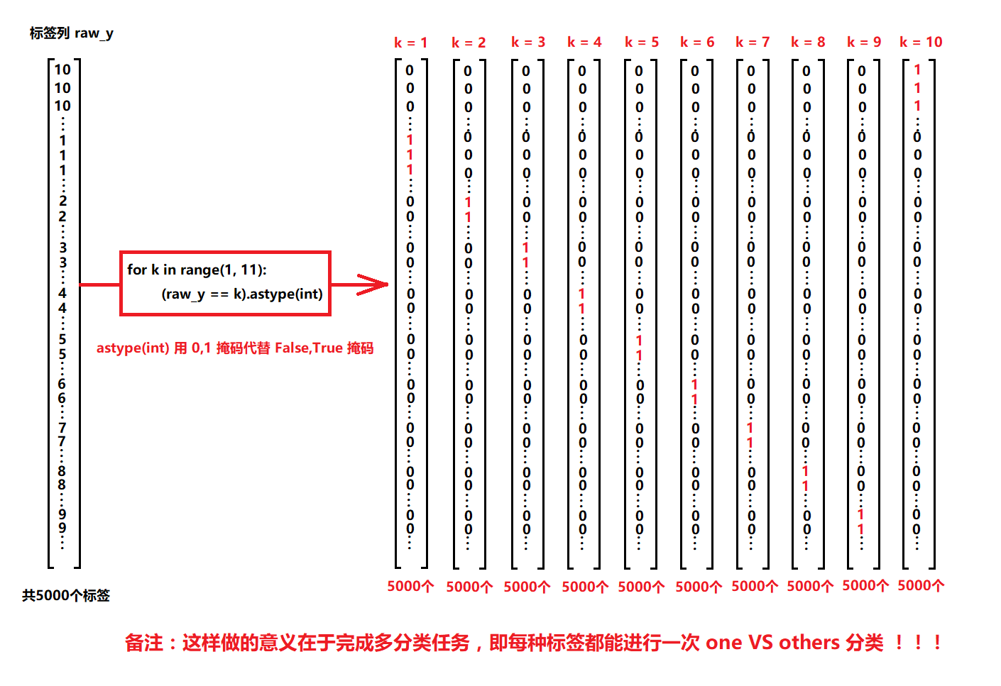
As shown in the figure above, the label data we obtained from the original dataset is a (5000,1) column vector.
Similarly, we refer to the second classification problem. There are only two kinds of labels for binary classification problems: 0 and 1.
When a is divided into a and B, we can convert the label corresponding to a to 1 and the label corresponding to other data to 0, and successfully separate a. A new label vector is obtained y 1 y_1 y1, containing only 0 and 1.
Similarly, we can use the same method to separate b, c and d. There should be three new label vectors y 2 , y 3 , y 4 y_2,y_3,y_4 y2,y3,y4.
This process is called the label vectorization process.
3. Multivariate classification process
- Read data
- Get eigenvalue X X X
- Get tag value y y y
- Tag value Vectorization y [ 0 ] , y [ 1 ] , y [ 2 ] , y [ 3 ] . . . y[0],y[1],y[2],y[3]... y[0],y[1],y[2],y[3]...
- Feature scaling (if necessary)
- Building functional relationships between features and labels (hypothetical functions)
- Constructing regularization cost function
- Find the partial derivative of the regularization cost function
- The minimum regularization cost function is used to obtain the weight at this time
- The functional relationship between features and labels is obtained according to the weight
The process of multivariate classification is only one more label value vectorization compared with the second classification, and the rest are exactly the same as the second classification. It should be noted that here y [ 0 ] y[0] y[0] is equivalent to a two classifier, which corresponds to a group θ [ 0 ] θ[0] θ [0], and y [ 1 ] y[1] y[1] is equivalent to another two classifier, which corresponds to a group θ [ 1 ] θ[1] θ [1] In this way, each label vector is equivalent to a two classifier, corresponding to a set of weight coefficients.
4. Difference between (n,) (n, 1)
One problem needs to be clarified before code implementation. This will help us understand the dimension correspondence related to calculation in the code.
numpy In, about(n,) (n,1)Differences between
We can observe the following code:
import numpy as np

list_1 = [[1, 2, 3]]
a = np.array(list_1)
print(a)  # [[1 2 3]]
print(a.shape)  # (1, 3)
b = np.arange(1, 4, 1).reshape(3, 1)
print(b)
# [[1]
#  [2]
#  [3]]
print(b.shape)   #(3, 1)
print(a @ b)  # [[14]]
# The calculation here is the calculation corresponding to the (1,3) (3,1) dimension, which is in line with our matrix calculation rules
import numpy as np

list_1 = [[1, 2, 3]]
a = np.array(list_1).reshape(3)
print(a)  # [1 2 3]
print(a.shape)  # (3,)
b = np.arange(1, 7, 1).reshape(3, 2)
print(b)
# [[1]
#  [2]
#  [3]]
print(b.shape)  # (3, 1)
print(a @ b)   # [14]
# We found that this code gives a result similar to the previous code. This is the calculation corresponding to the (3), (3,1) dimension. If it is based on the matrix calculation rules, can we understand it as follows:
# (3) row vector equivalent to (1,3)?
import numpy as np

list_1 = [[1, 2, 3]]
a = np.array(list_1).reshape(3)
print(a)  # [1 2 3]
print(a.shape)  # (3,)
b = np.arange(1, 4, 1).reshape(1,3)
print(b)  # [[1 2 3]]
print(b.shape)  # (1, 3)
print(b @ a)   # [14]
# In this code, we get the same result as in the second code. This is the calculation corresponding to the dimension (1,3) (3). If it is based on the matrix calculation rules, can we have the following understanding:
# (3) column vector equivalent to (3,1)?
# When we try to calculate (3), (1,3), we find that there is a syntax error
Through the above code, we get the following conclusions:
**(n,) when performing matrix operation, it can select whether it is expressed as column vector or row vector according to the situation. In this case, on the premise of following the matrix calculation rules, the calculation result must be a one-dimensional array, otherwise an error will be reported** Therefore, transforming (n,1) into (n,) can ignore the dimension correspondence to a certain extent.
5. Code implementation
5.1 graphical data
variable X X X ¢ sample pictures containing 5000 handwritten digits, each sample picture is 20 in size × 20 pixels, so each sample is represented as 400 dimensions, where the value represents the gray value of each pixel lattice.
variable y y y is the label corresponding to 5000 samples
In order to better understand the true meaning of the data, the data can be graphical through the following code:
import numpy as np
import scipy.io as sio
import matplotlib.pyplot as plt
import matplotlib


def load_data(path):  # Load data
    data = sio.loadmat(path)  # Read. mat data through path
    y = data.get('y')  # Get tag y(5000,1)
    y = y.reshape(y.shape[0])  # For the convenience of calculation, y is converted into a one-dimensional array of (5000,)
    X = data.get('X')  # (5000,400)
    return X, y


def plot_an_image(image):  # mapping
    fig, ax = plt.subplots(figsize=(1, 1))  # Define an image of size (1,1)
    ax.matshow(image.reshape((20, 20)), cmap=matplotlib.cm.binary)  # A function that draws a matrix or array into an image
    plt.xticks(np.array([]))   # The x-axis is not displayed
    plt.yticks(np.array([]))   # The y-axis is not displayed


X, raw_y = load_data('ex3data1.mat')  # Read feature X
pick_one = np.random.randint(0, 5000)  # Select a sample at random
print(pick_one)
plot_an_image(X[pick_one, :])  # Drawing according to the characteristics of selected samples, that is, drawing according to the gray value of pixel lattice
plt.show()
print('this should be {}'.format(raw_y[pick_one]))
Operation results:
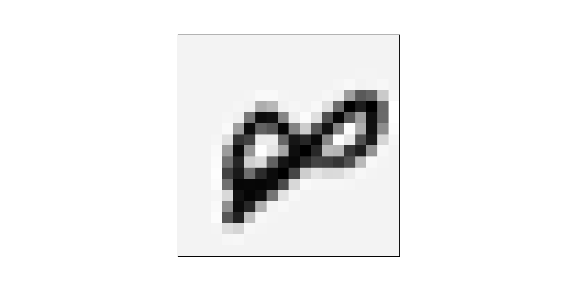
4004   # The 4004th sample
this should be 8
5.2 complete code
Because the process of multivariate classification is almost the same as that of binary classification, the code can be used simply by modifying the code of binary classification. The same code part as binary classification will not be commented in detail. For details, see Machine learning -- regularized logistic regression (classification) programming training Code comments in.
import numpy as np
import scipy.io as sio
import scipy.optimize as opt
from sklearn.metrics import classification_report  # This package is an evaluation report


def load_data(path):  # Load data
    data = sio.loadmat(path)  # Read. mat data through path
    y = data.get('y')  # Get tag y(5000,1)
    y = y.reshape(y.shape[0])  # For the convenience of calculation, y is converted into a one-dimensional array of (5000,)
    raw_X = data.get('X')  # (5000,400)
    X = np.insert(raw_X, 0, values=np.ones(raw_X.shape[0]), axis=1)  # The first column (all 1) is inserted, which is x_0 = 1
    return X, y


def label_vectorization(raw_y):  # Label Vectorization
    y_matrix = []  # Define an empty list to store vectorized data
    for k in range(1, 11):  # Label: 1-10, corresponding to 1-9 and 0, and the label is vectorized into 10 vectors
        y_matrix.append((raw_y == k).astype(int))
    y_matrix = [y_matrix[-1]] + y_matrix[:-1]  # Since the last vector corresponds to class 0, Class 0 is mentioned to the first, that is, 0-9
    y = np.array(y_matrix)  # Convert the list data type to the ndarray data type
    return y


def sigmoid(z):  # Define sigmoid function
    return 1 / (1 + np.exp(-z))


def cost(theta, X, y):  # To define the cost function, we need to pay attention to the dimensions of X, theta and y, which do not affect the calculation
    return np.mean(-y * np.log(sigmoid(X @ theta)) - (1 - y) * np.log(1 - sigmoid(X @ theta)))
    # It is worth mentioning that in numpy, +, -, *, / are only the operations of corresponding elements and do not follow the matrix calculation rules
    # Matrix calculation in numpy requires the use of @ or. dot() functions
    # Similarly, ndarray type data can be converted into a matrix through np.matrix() and calculated with *


def regularized_cost(theta, X, y, l=1):  # The regularization cost function l is the regularization coefficient
    theta_j1_to_n = theta[1:]  # from θ_ 1 to θ_ n. Usually, we are wrong θ_ 0 for regularization
    regularized_term = (l / (2 * len(X))) * np.power(theta_j1_to_n, 2).sum()  # The regular term of the cost function is a numerical value
    return cost(theta, X, y) + regularized_term


def gradient(theta, X, y):  # Partial derivative
    return (1 / len(X)) * X.T @ (sigmoid(X @ theta) - y)


def regularized_gradient(theta, X, y, l=1):  # The regularized partial derivative l is the regularization coefficient
    theta_j1_to_n = theta[1:]  # # from θ_ 1 to θ_ n
    regularized_theta = (l / len(X)) * theta_j1_to_n  # The regular term of partial derivative of cost function is an array
    # Because there is no regularization θ_ 0, so splice an array 0 to ensure the array dimension
    regularized_term = np.concatenate([np.array([0]), regularized_theta])
    return gradient(theta, X, y) + regularized_term


def logistic_regression(X, y, l=1):
    theta = np.zeros(X.shape[1])  # definition θ  To be the same as the feature data dimension
    # Using the optimization function in the optimizer, the TNC "truncated Newton method" is adopted
    res = opt.minimize(fun=regularized_cost,
                       x0=theta,
                       args=(X, y, l),
                       method='TNC',
                       jac=regularized_gradient)
    final_theta = res.x  # Get the final θ value
    return final_theta


def predict(x, theta):  # Prediction function
    prob = sigmoid(x @ theta)
    return (prob >= 0.5).astype(int)


# Get feature X, label y
X, raw_y = load_data('ex3data1.mat')
y = label_vectorization(raw_y)  # Label Vectorization

# logistic regression
k_theta = np.array([logistic_regression(X, y[k]) for k in range(10)])
# y[k].shape = (5000,) can be regarded as row vector and column vector
# k_theta.shape = (10,401)

# Prediction and verification
prob_matrix = sigmoid(X @ k_theta.T)  # h_ θ (x) , because it is composed of multiple two classifiers, it should be a matrix
# (5000401) [(10401). T] = = = > (5000,10), which means 5000 samples, and each sample belongs to the possibility of 0-9. The value with the greatest possibility is the predicted value.

y_pred = np.argmax(prob_matrix, axis=1)  # Returns the index of the maximum value along the axis. axis=1 represents the row. The index is 0-9, which better corresponds to the classification

y_ture = raw_y.copy()  # Tags 1-9 and 10 not vectorized
y_ture[y_ture == 10] = 0  # Replace 10 in the label with 0
print(classification_report(y_ture, y_pred))  # assessment report
6. Operation results
              precision    recall  f1-score   support

           0       0.97      0.99      0.98       500
           1       0.95      0.99      0.97       500
           2       0.95      0.92      0.93       500
           3       0.95      0.91      0.93       500
           4       0.95      0.95      0.95       500
           5       0.92      0.92      0.92       500
           6       0.97      0.98      0.97       500
           7       0.95      0.95      0.95       500
           8       0.93      0.92      0.92       500
           9       0.92      0.92      0.92       500

    accuracy                           0.94      5000
   macro avg       0.94      0.94      0.94      5000
weighted avg       0.94      0.94      0.94      5000
The recognition accuracy of 0 and 6 is very high, reaching 98% and 97%, while the recognition accuracy of 5 and 9 is low, only 92%. The overall recognition rate reached 94%.