1. Introduction
Target site: Jinjiang Literature City Library
Crawler Tool: BeautifulSoup
Data analysis: pandas, matplotlib
Word cloud: wordcloud, re
PS.Given that jj boss is very stubborn and has only three servers and only a few offices in the community, it is recommended to slow down the crawl speed by sleep when crawling to reduce the pressure on the server.
2. Reptiles
2.1 url parsing
Check any number of options on the first page of the database to try and see how the url changes (note the section outlined in the box):
-
Sex orientation: Emotions, sorted by publication time, show only completed url s:
https://www.jjwxc.net/bookbase.php?fw0=0&fbsj0=0&ycx0=0&[xx1=1]&mainview0=0&sd0=0&lx0=0&fg0=0&bq=&removebq=&[sortType=3]&collectiontypes=ors&searchkeywords=&[page=0]&[isfinish=2] -
Sex orientation: Pure love, sorted by collection of works, only shows unlimited, jump to page 4, get url:
https://www.jjwxc.net/bookbase.php?fw0=0&fbsj0=0&ycx0=0&[xx2=2]&mainview0=0&sd0=0&lx0=0&fg0=0&bq=&removebq=&[sortType=4]&[page=4]&[isfinish=0]&collectiontypes=ors&searchkeywords=
Several parameters are summarized:
- Pages: Page, starting from 1 (but 0 is also the first page). Upper limit is 1000.
- Sexual orientation: Emotion is xx1=1, pure love xx2=2, Lily xx3=3, if you want to choose more than one sexual orientation at the same time, write it together
- Sort by: sortType, update time = 1, collection = 4, publication time = 3, work credit = 2
- Is it finished: isfinish, unlimited = 0, in-line = 1, completed = 2
2.2 Page Element Resolution
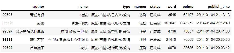
The data you want to crawl is as follows:
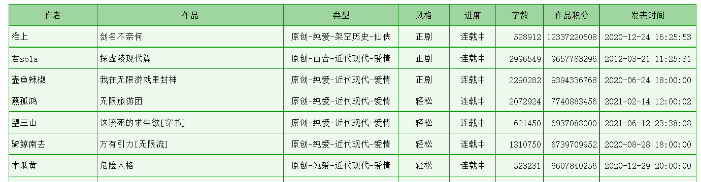
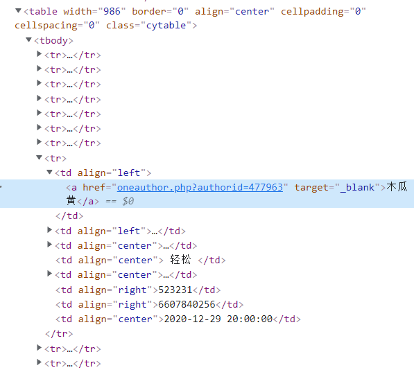
Press F12 to open the developer tool, look at the page elements, and find all the information in one table (class="cytable"), one tr per line and one td per cell.
2.3 Login
When you try to jump to more than 10 pages, an interface appears that requires you to log in:
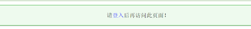
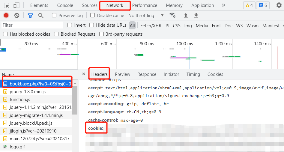
After login to Jinjiang account, press F12 to open the developer tool, open the network tab, refresh the page, find the corresponding package, copy the cookie in headers, and add it to the crawler's request header.
2.4 Complete Code
def main(save_path, sexual_orientation):
	"""
	save_path: File Save Path
    sexual_orientation: 1: Emotions, 2: pure love, 3: lily, 4: female dignity, 5: none CP
    """
    for page in range(1, 1001):
        url = get_url(page, sexual_orientation)
        headers = {
            'cookie': Your cookie,
            'User-Agent': 'Mozilla/5.0 (Windows NT 10.0; Win64; x64) AppleWebKit/537.36 (KHTML, like Gecko) Chrome/93.0.4577.63 Safari/537.36'}
        html = requests.get(url, headers=headers)
        html.encoding = html.apparent_encoding
        try:
            data = parse(html.content)
        except:
            print("Crawl failed:", page)
            continue
        if len(data) == 0:
            break
        df = pd.DataFrame(data)
        df.to_csv(save_path, mode='a', header=False, index=False)
        print(page)
        time.sleep(3)


def get_url(page, sexual_orientation):
    url = f"https://www.jjwxc.net/bookbase.php?fw0=0&fbsj0=0&ycx1=1&xx{sexual_orientation}={sexual_orientation}&mainview0=0&sd0=0&lx0=0&fg0=0&bq=-1&" \
          f"sortType=3&isfinish=2&collectiontypes=ors&page={page}"
    return url


def parse(document):
    soup = BeautifulSoup(document, "html.parser")
    table = soup.find("table", attrs={'class': 'cytable'})
    rows = table.find_all("tr")
    data_all = []
    for row in rows[1:]:
        items = row.find_all("td")
        data = []
        for item in items:
            text = item.get_text(strip=True)
            data.append(text)
        data_all.append(data)
    return data_all

if __name__ == "__main__":
	main("Emotions.txt", 1)
3.Data analysis and visualization
Use pandas to read the crawled data as follows:
Simple preprocessing
# Duplicate removal
df = df.drop_duplicates(subset=["author", "name"])
print("Number of articles:", df.shape[0])

# Time Type Conversion
df["publish_time"] = pd.to_datetime(df["publish_time"])

# Convert Word Count to Ten Thousand Words
df["word"] /= 10000

# Integral converted to ten thousand
df["points"] /= 10000
3.1 Column
View the minimum and maximum number of words:
df["word"].min(), df["word"].max()
Results: (0.0001, 616.9603) (unit: 10,000 words), so the minimum value was set to 0 and the maximum value was set to 700 when grouping.
# Set the location of data grouping
bins_words = [0, 0.5, 1, 10, 20, 40, 60, 80, 100, 700]
# Distribution of Words in Novels Published Before 2018
words_distribution1 = pd.value_counts(pd.cut(df.query("publish_time<'2018-01-01'")["word"], bins=bins_words), sort=False)
words_distribution1 /= np.sum(words_distribution1) # normalization
# Distribution of Words in Novels Published After 2018
words_distribution2 = pd.value_counts(pd.cut(df.query("publish_time>='2018-01-01'")["word"], bins=bins_words), sort=False)
words_distribution2 /= np.sum(words_distribution2) # normalization
# Drawing
plt.figure(dpi=100)
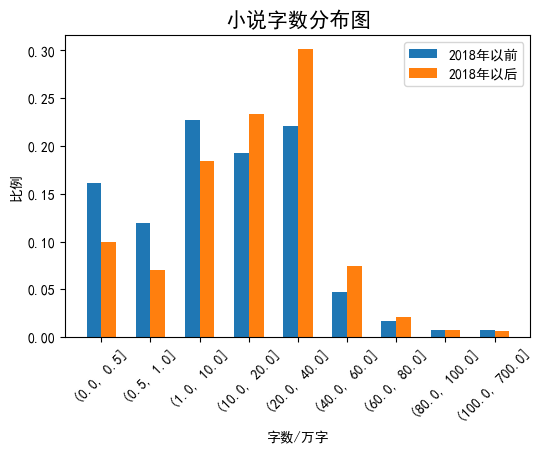
plt.title("Fiction Word Number Distribution Map", fontsize=15)
loc = np.array([i for i in range(len(words_distribution1.index))])
plt.bar(loc-0.15, words_distribution1.values, width=0.3, label="2018 Years ago")
plt.bar(loc+0.15, words_distribution2.values, width=0.3, label="2018 Year later")
plt.xticks(loc, words_distribution1.index, rotation=45)
plt.xlabel("Number of words/Ten thousand words")
plt.ylabel("Proportion")
plt.legend()
3.2 Pie Chart
- Type statistics.
Most types of formats are "Origin - Pure Love - Overhead History - Fairy Man", which can be split at intervals of "-" with a third tag.
However, there are a small number of works whose type format is "essays"/"comments"/"unknown". Direct access to elements marked 2 will result in errors, so an if statement is added to process them.# Type Statistics tags = df["type"].apply(lambda x: x.split("-")[2] if len(x.split("-"))==4 else x) tag_count = pd.value_counts(tags) # Categories with too few merges tag_count["Other"] = tag_count["Unknown"] + tag_count["Informal essay"] + tag_count["comment"] + tag_count["Poetry"] + tag_count[""] tag_count = tag_count.drop(["Unknown","Informal essay","comment","Poetry", ""]) - Style Statistics
# Style Statistics
manner_count = pd.value_counts(df["manner"])

# Categories with too few merges
manner_count["Other"] = manner_count["Dark"] + manner_count["Laughing"] + manner_count["Unknown"]
manner_count = manner_count.drop(["Dark", "Laughing", "Unknown"])
- Drawing
fig, axes = plt.subplots(1, 2, figsize=(10,5), dpi=100)
fig.subplots_adjust(wspace=0.05)
axes[0].pie(tag_count,
        labels=tag_count.index,
        autopct='%1.2f%%',
        pctdistance=0.7,
        colors=[plt.cm.Set3(i) for i in range(len(tag_count))],
        textprops={'fontsize':10},
        wedgeprops={'linewidth': 1, 'edgecolor': "black"}
       )
axes[0].set_title("type", fontsize=15)

axes[1].pie(manner_count,
        labels=manner_count.index,
        autopct='%1.2f%%',
        pctdistance=0.7,
        colors=[plt.cm.Accent(i) for i in range(len(manner_count))],
        textprops={'fontsize':10},
        wedgeprops={'linewidth': 1, 'edgecolor': "black"}
       )
axes[1].set_title("style", fontsize=15)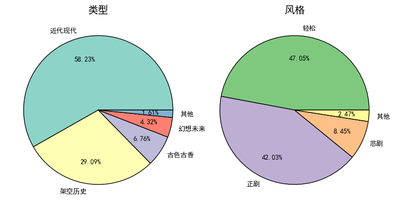
4.Story Title Ci Cloud
from wordcloud import WordCloud
import jieba
import pandas as pd
import matplotlib.pyplot as plt
import re
4.1 participle
- Main points:
- Separate each title using the jieba thesaurus (Vectorization with DataFrame speeds up processing)
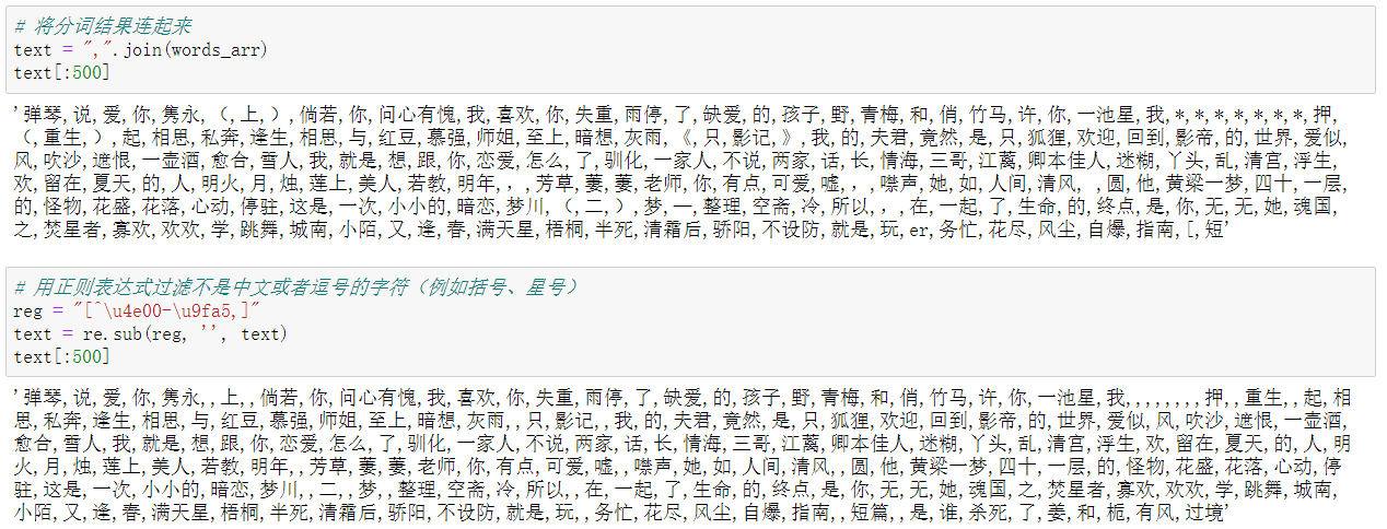
- The original title contains more symbols (e.g. (top), [ABO], the * symbol changed by crab), and English characters, which can be removed using regular expressions.
Before removal vs after removal:
- Code:
# Add Custom Words
jieba.add_word("Fast Wear")
# Separate each title, separated by English commas
words_arr = df["name"].apply(lambda x: ",".join(jieba.cut(x))).values
# Connect the participle results
text = ",".join(words_arr)
# Filter characters (such as brackets, asterisks) that are not Chinese or commas with regular expressions
reg = "[^\u4e00-\u9fa5,]"
text = re.sub(reg, '', text)
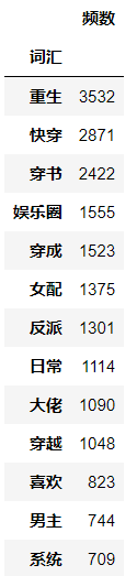
4.2 Word Frequency Statistics
-
Main points
- Word Frequency Statistics Using DataFrame
- Empty strings (products of regular symbol removal) and large numbers of words found in high frequency vocabulary are meaningless for data analysis and need to be removed.
Before removal After removal 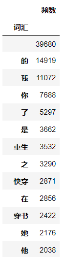
-
Code
# word frequency count
words_list = text.split(",")
df_freq = pd.DataFrame(pd.value_counts(words_list), columns=["frequency"])
df_freq.index.name="vocabulary"
# Remove Words
stop_words = df_freq[df_freq.index.str.len()<=1].index.tolist()
df_freq = df_freq[df_freq.index.str.len()>1]
# Visualization of Top Vocabularies
plt.figure(figsize=(15, 5))
x = [i for i in range(20)]
y = df_freq.iloc[:20].values.flatten()
labels = df_freq.index[:20]
plt.bar(x, y, color='steelblue', width=0.5)
plt.xticks(ticks=x, labels=labels, fontsize=15, rotation=45)
plt.title("Title of Jinjiang Literature City's Novels Top20 Popular Words", fontsize=15)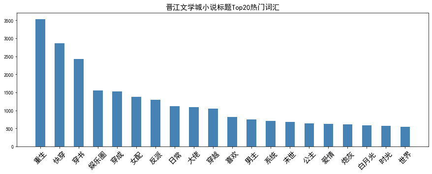
4.3 Word Cloud Visualization
- Main points
- Mask: An 8-bit gray-scale logo of Jinjiang Literature City is used as the mask. Essentially, it is a two-dimensional matrix with a partial value of 0 and a partial value of 1. Other pictures, such as RGB format, can be converted by themselves according to this rule.
- Stop word: Use the word removed from the word frequency statistics as a stop word.

- Code
# Generate Mask
mask = plt.imread(r"D:\2021 Grind first\Geographic information visualization\data\logo.bmp")
wordcloud = WordCloud(font_path=r"C:\Windows\Fonts\simhei.ttf",
                      stopwords=stop_words,
                      width=800, height=600,
                      mask=mask,
                      max_font_size=150,
                      mode='RGBA', background_color=None).generate(text)
fig = plt.figure(figsize=(10, 10))
ax = fig.add_subplot(111)
ax.axis("off")
ax.imshow(wordcloud, interpolation='bilinear')
plt.tight_layout(pad=4.5)
fig.savefig("wordcloud.png")