Author home page( Silicon based workshop of slow fire rock sugar): Slow fire rock sugar (Wang Wenbing) blog silicon based workshop of slow fire rock sugar _csdnblog
Website of this article: https://blog.csdn.net/HiWangWenBing/article/details/120600621
catalogue
Introduction deep learning model framework
Chapter 1 business area analysis
one point one Step 1-1: business domain analysis
1.2 steps 1-2: Business Modeling
1.3 code instance preconditions
Chapter 2 definition of forward operation model
two point one Step 2-1: dataset selection
two point two Step 2-2: Data Preprocessing
2.3 step 2-3: neural network modeling
2.4 steps 2-4: neural network output
Chapter 3 definition of backward operation model
3.1 step 3-1: define the loss function
three point two Step 3-2: define the optimizer
3.4 step 3-4: model validation
3.5 step 3-5: Model Visualization
4.1 step 4-1: model deployment
Introduction deep learning model framework
 https://blog.csdn.net/HiWangWenBing/article/details/120462734
Chapter 1 business area analysis
one point one Step 1-1: business domain analysis
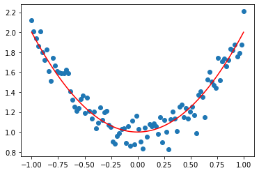
Nonlinear regression, samples are noisy data.
It can be seen from the sample data that the internal law may be a parabola, but it must be a univariate function (straight line)
Therefore, this is a nonlinear regression problem.
1.2 steps 1-2: Business Modeling
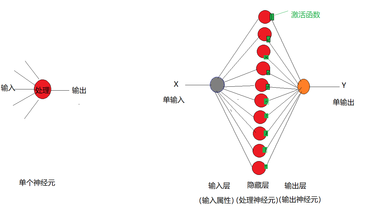
A single neuron is both an input and a single output.
Two layers of neural networks can be constructed:
(1) Hidden layer 1:
- One dimensional input attribute X
- Multiple parallel neurons, 10 neurons are preliminarily selected here
- Each neuron has an activation function relu
(2) Output layer:
- Because it is a single input, only one neuron is needed in the output layer.
1.3 code instance preconditions
#Environmental preparation
import numpy as np              # numpy array library
import math                     # Mathematical operation Library
import matplotlib.pyplot as plt # Drawing library

import torch             # torch base library
import torch.nn as nn    #  torch neural network library
import torch.nn.functional as F    #  torch neural network library

print("Hello World")
print(torch.__version__)
print(torch.cuda.is_available())
Hello World 1.8.0 False
Chapter 2 definition of forward operation model
two point one Step 2-1: dataset selection
There is no need to use the existing open source data set, just build the data set yourself.
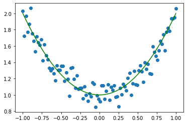
#2-1 preparing data sets
#x_sample = torch.linspace(-1, 1, 100).reshape(-1, 1) or
x_sample = torch.unsqueeze(torch.linspace(-1, 1, 100), dim=1)

#The noise obeys normal distribution
noise = torch.randn(x_sample.size())

y_sample = x_sample.pow(2) + 1 + 0.1 * noise

y_line =   x_sample.pow(2) + 1

#Visual data
print(x_sample.shape)
print(y_sample.shape)
print(y_line.shape)
plt.scatter(x_sample.data.numpy(), y_sample.data.numpy())
plt.plot(x_sample, y_line,'green')
torch.Size([100, 1])
torch.Size([100, 1])
torch.Size([100, 1])
Out[51]:
[<matplotlib.lines.Line2D at 0x279b8d43130>]
two point two Step 2-2: Data Preprocessing
# 2-2 data preprocessing
x_train = x_sample
y_train = y_sample
2.3 step 2-3: neural network modeling
# 2-3 define network model
class Net(torch.nn.Module):
    # Defining neural networks
    def __init__(self, n_feature, n_hidden, n_output):
        super(Net, self).__init__()
        #Define hidden layer L1
        # n_feature: enter the dimension of the attribute
        # n_hidden: number of neurons = number of output attributes
        self.hidden = torch.nn.Linear(n_feature, n_hidden)

        #Define output layer:
        # n_hidden: enter the dimension of the attribute
        # n_output: number of neurons = number of output attributes
        self.predict = torch.nn.Linear(n_hidden, n_output)

    #Define forward operation
    def forward(self, x):
        h1  = self.hidden(x)
        s1  = F.relu(h1)
        out = self.predict(s1)
        return out

model = Net(1,10,1)
print(model)
print(model.parameters)
print(model.parameters())
Net( (hidden): Linear(in_features=1, out_features=10, bias=True) (predict): Linear(in_features=10, out_features=1, bias=True) ) <bound method Module.parameters of Net( (hidden): Linear(in_features=1, out_features=10, bias=True) (predict): Linear(in_features=10, out_features=1, bias=True) )> <generator object Module.parameters at 0x00000279B78BC820>
2.4 steps 2-4: neural network output
# 2-4 define network prediction output
y_pred = model.forward(x_train)
print(y_pred.shape)
torch.Size([100, 1])
Chapter 3 definition of backward operation model
3.1 step 3-1: define the loss function
The MSE loss function used here
# 3-1 define the loss function:
# loss_fn= MSE loss
loss_fn = nn.MSELoss()

print(loss_fn)
MSELoss()
three point two Step 3-2: define the optimizer
# 3-2 defining the optimizer
Learning_rate = 0.01     #Learning rate

# optimizer = SGD: basic gradient descent method
# Parameters: indicates the list of parameters to be optimized
# lr: indicates the learning rate
optimizer = torch.optim.SGD(model.parameters(), lr = Learning_rate)
print(optimizer)
SGD (
Parameter Group 0
    dampening: 0
    lr: 0.01
    momentum: 0
    nesterov: False
    weight_decay: 0
)
3.3 step 3-3: model training
# 3-3 model training
# Define the number of iterations
epochs = 10000

loss_history = [] #loss data during training

for i in range(0, epochs):

    #(1) Forward calculation
    y_pred = model(x_train)

    #(2) Calculate loss
    loss = loss_fn(y_pred, y_train)

    #(3) Reverse derivation
    loss.backward()

    #(4) Reverse iteration
    optimizer.step()

    #(5) Reset the gradient of the optimizer
    optimizer.zero_grad()

    # Record training data
    loss_history.append(loss.item())

    if(i % 1000 == 0):
        print('epoch {}  loss {:.4f}'.format(i, loss.item()))

print("\n Iteration completion")
print("final loss =", loss.item())
print(len(loss_history))
epoch 0 loss 1.9343 epoch 1000 loss 0.0152 epoch 2000 loss 0.0119 epoch 3000 loss 0.0115 epoch 4000 loss 0.0111 epoch 5000 loss 0.0108 epoch 6000 loss 0.0105 epoch 7000 loss 0.0103 epoch 8000 loss 0.0102 epoch 9000 loss 0.0101 Iteration completion final loss = 0.010022741742432117 10000
3.4 step 3-4: model validation
NA
3.5 step 3-5: Model Visualization
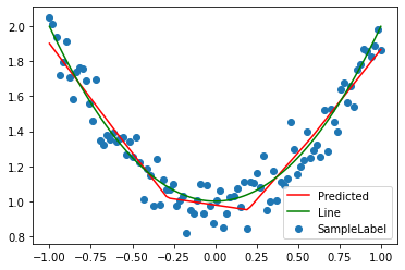
(1) Forward data
# 3-5 visual model data
#The model returns the total tensors, including grad_fn. The tensors extracted from data are pure tensors
y_pred = model.forward(x_train).data.numpy().squeeze()
print(x_train.shape)
print(y_pred.shape)
print(y_line.shape)

plt.scatter(x_train, y_train, label='SampleLabel')
plt.plot(x_train, y_pred, color ="red", label='Predicted')
plt.plot(x_train, y_line, color ="green", label ='Line')

plt.legend()
plt.show()
torch.Size([100, 1])
(100,)
torch.Size([100, 1])
(2) Backward loss iterative process
#Display historical data of loss
plt.plot(loss_history, "r+")
plt.title("loss value")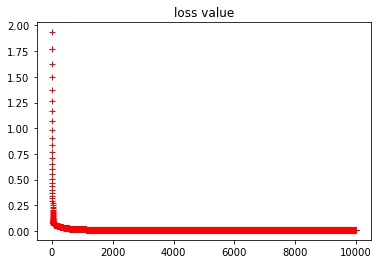
Chapter 4 model deployment
4.1 step 4-1: model deployment
NA
Author home page( Silicon based workshop of slow fire rock sugar): Slow fire rock sugar (Wang Wenbing) blog silicon based workshop of slow fire rock sugar _csdnblog
Website of this article: https://blog.csdn.net/HiWangWenBing/article/details/120600621