In the actual process of building neural network, forward propagation is easy to realize and has high correctness; The implementation of back propagation is difficult, and there are often bug s. For items requiring high accuracy, gradient test is particularly important.
Principle of gradient test
The definition of derivative (gradient) in mathematics is
∂
J
∂
θ
=
lim
ε
→
0
J
(
θ
+
ε
)
−
J
(
θ
−
ε
)
2
ε
\frac{\partial J}{\partial \theta} =\lim_{\varepsilon \to 0} \frac{J(\theta + \varepsilon) - J(\theta - \varepsilon)}{2\varepsilon}
∂θ∂J=ε→0lim2εJ(θ+ε)−J(θ−ε)
We need to verify the results of back propagation calculation
∂
J
∂
θ
\frac{\partial J}{\partial \theta}
∂ θ ∂ J ∂ can be calculated by forward propagation in another way, that is, the above formula
J
(
θ
+
ε
)
J(\theta + \varepsilon)
J( θ+ε) and
J
(
θ
−
ε
)
J(\theta - \varepsilon)
J( θ − ε) To get
∂
J
∂
θ
\frac{\partial J}{\partial \theta}
∂ θ ∂ J, verify whether it is the same as that calculated by back propagation.
Python implementation of gradient test
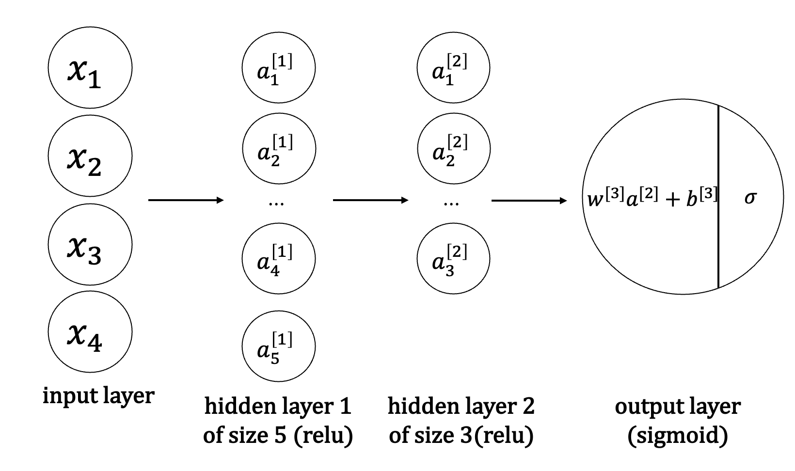
We simply build a 3-layer neural network, as shown in the figure below
def gradient_check_n_test_case():
    np.random.seed(1)
    x = np.random.randn(4,3)
    y = np.array([1, 1, 0])
    W1 = np.random.randn(5,4)
    b1 = np.random.randn(5,1)
    W2 = np.random.randn(3,5)
    b2 = np.random.randn(3,1)
    W3 = np.random.randn(1,3)
    b3 = np.random.randn(1,1)
    parameters = {"W1": W1,
                  "b1": b1,
                  "W2": W2,
                  "b2": b2,
                  "W3": W3,
                  "b3": b3}


    return x, y, parameters
Realize its forward propagation and back propagation respectively (two errors are deliberately added in the back propagation)
def forward_propagation_n(X, Y, parameters):
    m = X.shape[1]
    W1 = parameters["W1"]
    b1 = parameters["b1"]
    W2 = parameters["W2"]
    b2 = parameters["b2"]
    W3 = parameters["W3"]
    b3 = parameters["b3"]

    # RELU -> RELU -> SIGMOID
    Z1 = np.dot(W1, X) + b1
    A1 = relu(Z1)
    Z2 = np.dot(W2, A1) + b2
    A2 = relu(Z2)
    Z3 = np.dot(W3, A2) + b3
    A3 = sigmoid(Z3)

    logprobs = np.multiply(-np.log(A3), Y) + np.multiply(-np.log(1 - A3), 1 - Y)
    cost = 1. / m * np.sum(logprobs)

    cache = (Z1, A1, W1, b1, Z2, A2, W2, b2, Z3, A3, W3, b3)

    return cost, cache


def backward_propagation_n(X, Y, cache):
    m = X.shape[1]
    (Z1, A1, W1, b1, Z2, A2, W2, b2, Z3, A3, W3, b3) = cache

    dZ3 = A3 - Y
    dW3 = 1. / m * np.dot(dZ3, A2.T)
    db3 = 1. / m * np.sum(dZ3, axis=1, keepdims=True)

    dA2 = np.dot(W3.T, dZ3)
    dZ2 = np.multiply(dA2, np.int64(A2 > 0))
    dW2 = 1. / m * np.dot(dZ2, A1.T) * 2  # Error 1
    db2 = 1. / m * np.sum(dZ2, axis=1, keepdims=True)

    dA1 = np.dot(W2.T, dZ2)
    dZ1 = np.multiply(dA1, np.int64(A1 > 0))
    dW1 = 1. / m * np.dot(dZ1, X.T)
    db1 = 4. / m * np.sum(dZ1, axis=1, keepdims=True)  # Error 2

    gradients = {"dZ3": dZ3, "dW3": dW3, "db3": db3,
                 "dA2": dA2, "dZ2": dZ2, "dW2": dW2, "db2": db2,
                 "dA1": dA1, "dZ1": dZ1, "dW1": dW1, "db1": db1}

    return gradients
We pass a one-dimensional column vector
g
r
a
d
a
p
p
r
o
x
gradapprox
Gradaprox preserves the gradient obtained by forward propagation, and each element corresponds to the gradient of a parameter
g
r
a
d
grad
grad is compared with it to judge whether the error is too large.
The formula for calculating the comparison is
d
i
f
f
e
r
e
n
c
e
=
∥
g
r
a
d
−
g
r
a
d
a
p
p
r
o
x
∥
2
∥
g
r
a
d
∥
2
+
∥
g
r
a
d
a
p
p
r
o
x
∥
2
difference = \frac{\left \|grad - gradapprox \right \| _2}{\left \|grad \right \| _2+\left \|gradapprox \right \| _2}
difference=∥grad∥2+∥gradapprox∥2∥grad−gradapprox∥2
numpy's norm function is used to calculate the norm of the matrix.
def gradient_check_n(parameters, gradients, X, Y, epsilon=1e-7):
parameters_values, _ = dictionary_to_vector(parameters)
grad = gradients_to_vector(gradients)
num_parameters = parameters_values.shape[0]
J_plus = np.zeros((num_parameters, 1))
J_minus = np.zeros((num_parameters, 1))
gradapprox = np.zeros((num_parameters, 1))
# Calculate gradaprox
for i in range(num_parameters):
thetaplus = np.copy(parameters_values)
thetaplus[i][0] = thetaplus[i][0] + epsilon
J_plus[i], _ = forward_propagation_n(X, Y, vector_to_dictionary(thetaplus))
thetaminus = np.copy(parameters_values)
thetaminus[i][0] = thetaminus[i][0] - epsilon
J_minus[i], _ = forward_propagation_n(X, Y, vector_to_dictionary(thetaminus))
gradapprox[i] = (J_plus[i] - J_minus[i]) / (2 * epsilon)
numerator = np.linalg.norm(grad - gradapprox)
denominator = np.linalg.norm(grad) + np.linalg.norm(gradapprox)
difference = numerator / denominator
if difference < 2e-7:
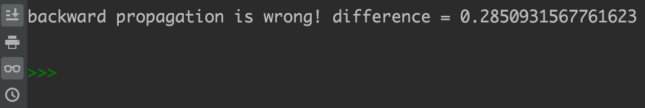
print("backward propagation is wrong! difference = " + str(difference))
else:
print("backward propagation is right! difference = " + str(difference))
return difference
The operation results are as follows
X, Y, parameters = gradient_check_n_test_case()

cost, cache = forward_propagation_n(X, Y, parameters)
gradients = backward_propagation_n(X, Y, cache)
difference = gradient_check_n(parameters, gradients, X, Y)
For the complete code of this experiment, see:
https://github.com/PPPerry/AI_projects/tree/main/6.gradient_check
Tips
- The gradient test is very slow. Using an approximate formula to calculate the gradient is very computationally expensive. It can only be turned on when it is necessary to verify whether the code is correct. After confirming that the code is OK, turn off the gradient test.
- Gradient test cannot coexist with dropout.
Previous AI series experiments:
A series of artificial intelligence experiments (I) -- binary classification single layer neural network for cat recognition
Series of artificial intelligence experiments (II) -- shallow neural network for distinguishing different color regions
Series of experiments on artificial intelligence (III) -- binary classification depth neural network for cat recognition
Series of experiments on artificial intelligence (IV) -- comparison of various neural network parameter initialization methods (Xavier initialization and He initialization)
Series of experiments on artificial intelligence (V) -- regularization method: Python implementation of L2 regularization and dropout