1, Theoretical basis

1. Node coverage model

0 / 1 coverage model is adopted in this paper. Please refer to for specific description here.

2. Symbiotic biological search algorithm (SOS)

SOS algorithm imitates biological behavior, and finally forms three evolutionary stages of "mutually beneficial symbiosis", "favorable symbiosis" and "parasitism", guiding individuals to evolve gradually. The key operations of SOS algorithm are as follows:

(1) Population initialization

Suppose the population number is N N N. The upper and lower limits of individual search range are respectively U U U and L L 50. Generate randomly according to the following formula N N N initial individuals X i X_i Xi​: X i = L + rand ( 1 , D ) × ( U − L ) (1) X_i=L+\text{rand}(1,D)×(U-L)\tag{1} Xi​=L+rand(1,D) × (U − L)(1) where, X i X_i Xi ， represents the second in the population i i i( i = 1 , 2 , ⋯   , N i=1,2,\cdots,N i=1,2,..., N) biological individuals, rand \text{rand} rand representation [ 0 , 1 ] [0,1] Random number between [0,1], D D D represents the dimension of the optimized problem.

(2) Mutually beneficial symbiosis

For each individual in the population X i X_i Xi, randomly select one other individual X j ( i , j ∈ { 1 , 2 , ⋯   , N } , j ≠ i ) X_j(i, j\in\{1,2,\cdots,N\},j≠i) Xj (i,j ∈ {1,2,..., N},j  = i) and itself
Through mutually beneficial symbiosis, 2 new individuals are generated: { X i new = X i + rand ( 0 , 1 ) × ( X best − MV × BF 1 ) X j new = X j + rand ( 0 , 1 ) × ( X best − MV × BF 2 ) (2) \begin{dcases}X_{i\text{new}}=X_i+\text{rand}(0,1)×(X_{\text{best}}-\text{MV}×\text{BF}_1)\\X_{j\text{new}}=X_j+\text{rand}(0,1)×(X_{\text{best}}-\text{MV}×\text{BF}_2)\end{dcases}\tag{2} {Xinew​=Xi​+rand(0,1) × (Xbest​−MV × BF1​)Xjnew​=Xj​+rand(0,1) × (Xbest​−MV × BF2) (2) where, rand ( 0 , 1 ) \text{rand}(0,1) rand(0,1) is [ 0 , 1 ] [0,1] Random number between [0,1]; X best X_{\text{best}} Xbest ， is the optimal individual under the current number of iterations; MV = ( X i + X j ) / 2 \text{MV}=(X_i+X_j)/2 MV=(Xi + Xj) / 2 is "mutually beneficial vector", representing the relationship characteristics between organisms; BF 1 \text{BF}_1 BF1​, BF 2 \text{BF}_2 BF2 ￠ is the benefit factor, and 1 or 2 is randomly selected.
A new individual is generated by formula (2) X i new X_{i_\text{new}} Xinew # and X j new X_{j_\text{new}} Xjnew, through and X i X_i Xi # and X j X_j Xj) compare the fitness values and retain them finally X i new X_{i_\text{new}} Xinew ， and X i X_i Xi​, X j new X_{j_\text{new}} Xjnew and X j X_j The better individual in Xj ， is replaced X i X_i Xi # and X j X_j Xj​.

(3) Partial benefit symbiosis

Individuals in the population X i X_i Xi ， carry out the strategy of "partial benefit symbiosis" according to the following formula: X i new = X i + rand ( − 1 , 1 ) × ( X best − X j ) (3) X_{i\text{new}}=X_i+\text{rand}(-1,1)×(X_{\text{best}}-X_j)\tag{3} Xinew​=Xi​+rand(−1,1) × (Xbest − Xj) (3) where, X j X_j Xj ＾ is the population with X i X_i Xi) different individuals, i.e i , j ∈ { 1 , 2 , ⋯   , N } , j ≠ i i,j\in\{1,2,\cdots,N\},j≠i i,j∈{1,2,⋯,N},j​=i； X best X_{\text{best}} Xbest ， is the optimal individual in the current population; rand ( − 1 , 1 ) \text{rand}(-1,1) rand(− 1,1) is [ − 1 , 1 ] [-1,1] A random number between [− 1,1]. An individual newly generated by equation (3) X i new X_{i\text{new}} Xinew decides whether to replace after comparing the fitness values X i X_i Xi​.
It can be seen from the strategy of partial benefit symbiosis: similar to the "mutually beneficial symbiosis" stage, each individual randomly selects one other individual from the population to interact with itself; the difference is that the interaction between the two only makes X i X_i Xi # benefits for X j X_j Xj) its own development has neither interests nor harm.

(4) Parasitism

Generate one or more random numbers (no more than the number of gene loci) in the definition domain and modify the individual X i X_i Xi ＾ corresponding loci to form new individuals Parasite_Vector \text{Parasite\_Vector} Parasite_vector (p_v for short), and randomly selected individuals X j ( i , j ∈ 1 , 2 , ⋅ ⋅ ⋅ , N , j ≠ i ) X_j(i, j∈ {1,2,· · ·, N}, j≠i) Xj (i,j ∈ 1,2, ⋅⋅⋅, N,j  = I) (called "host") for fitness value comparison. If the fitness value of P_V is better, then "host" X j X_j Xj # will be replaced by P_V, otherwise X j X_j Xj ， will be considered as immune individuals to be retained.

2, Simulation experiment and analysis

1. Function test and numerical analysis

SOS is compared with FPA, WOA, MFO, SCA and GWO. Taking F1, F2, F16, F17, F25 and F26 in literature [1] as examples, the population size is set to 30, the maximum number of iterations is set to 500, and each algorithm operates 30 times independently. The results are shown as follows:

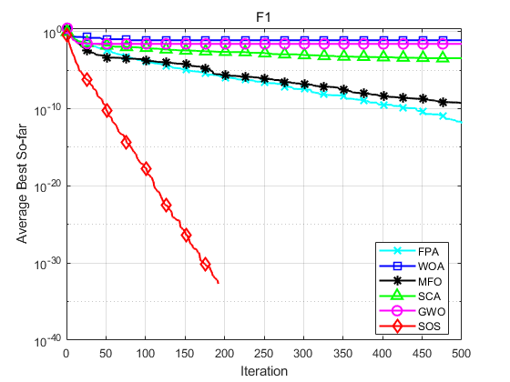
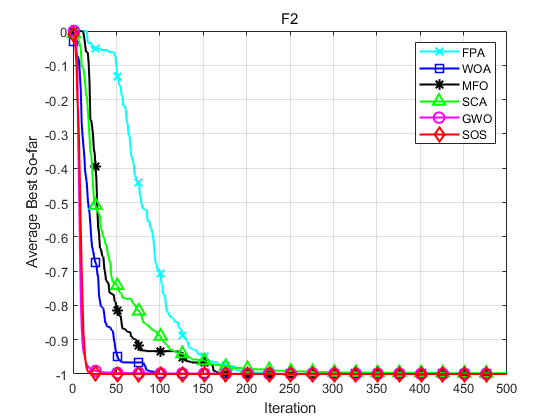
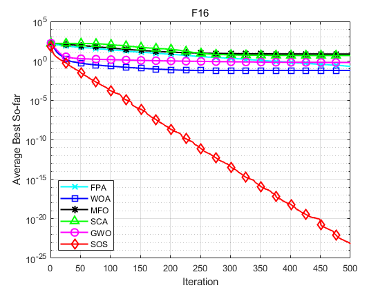
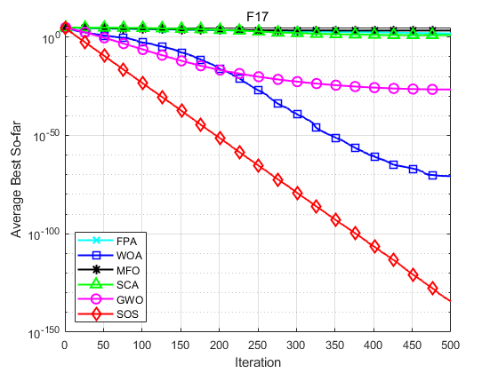
Function: F1
FPA: Worst value: 9.5109e-12,optimal value:1.1937e-18,average value:1.2781e-12,standard deviation:2.4481e-12
WOA: Worst value: 0.76207,optimal value:2.3163e-13,average value:0.076207,standard deviation:0.23253
MFO: Worst value: 1.6904e-08,optimal value:0,average value:5.6347e-10,standard deviation:3.0863e-09
SCA: Worst value: 0.0029332,optimal value:1.1219e-05,average value:0.00034985,standard deviation:0.0005416
GWO: Worst value: 0.76207,optimal value:3.8961e-09,average value:0.025402,standard deviation:0.13913
SOS: Worst value: 0,optimal value:0,average value:0,standard deviation:0
 Function: F2
FPA: Worst value: -1,optimal value:-1,average value:-1,standard deviation:4.0834e-09
WOA: Worst value: -1,optimal value:-1,average value:-1,standard deviation:6.8516e-07
MFO: Worst value: -1,optimal value:-1,average value:-1,standard deviation:0
SCA: Worst value: -0.99207,optimal value:-0.99989,average value:-0.9979,standard deviation:0.0020357
GWO: Worst value: -1,optimal value:-1,average value:-1,standard deviation:8.2047e-07
SOS: Worst value: -1,optimal value:-1,average value:-1,standard deviation:0
 Function: F16
FPA: Worst value: 0.4289,optimal value:0.087323,average value:0.20346,standard deviation:0.075546
WOA: Worst value: 0.15936,optimal value:0.024134,average value:0.061615,standard deviation:0.037101
MFO: Worst value: 42.6906,optimal value:0.001229,average value:7.4352,standard deviation:13.1045
SCA: Worst value: 6.976,optimal value:3.7828,average value:4.8192,standard deviation:0.61568
GWO: Worst value: 1.2637,optimal value:6.5089e-05,average value:0.62033,standard deviation:0.30985
SOS: Worst value: 5.5871e-23,optimal value:1.1133e-26,average value:6.7267e-24,standard deviation:1.3362e-23
 Function: F17
FPA: Worst value: 130.5562,optimal value:37.1901,average value:68.9236,standard deviation:24.3054
WOA: Worst value: 5.9377e-70,optimal value:2.1857e-89,average value:1.9822e-71,standard deviation:1.084e-70
MFO: Worst value: 10001.9982,optimal value:0.66141,average value:2006.8331,standard deviation:4065.0722
SCA: Worst value: 68.3455,optimal value:0.0017531,average value:10.2897,standard deviation:17.2873
GWO: Worst value: 1.278e-26,optimal value:3.4061e-29,average value:2.0882e-27,standard deviation:3.1648e-27
SOS: Worst value: 1.0245e-133,optimal value:5.2837e-139,average value:4.0699e-135,standard deviation:1.8616e-134
 Function: F25
FPA: Worst value: 2.3744,optimal value:1.3128,average value:1.6881,standard deviation:0.24307
WOA: Worst value: 0,optimal value:0,average value:0,standard deviation:0
MFO: Worst value: 90.8951,optimal value:0.3891,average value:16.0292,standard deviation:33.9355
SCA: Worst value: 1.473,optimal value:0.17989,average value:0.91643,standard deviation:0.34017
GWO: Worst value: 0.042361,optimal value:0,average value:0.0051044,standard deviation:0.009838
SOS: Worst value: 0,optimal value:0,average value:0,standard deviation:0
 Function: F26
FPA: Worst value: 16.5721,optimal value:6.0727,average value:10.7366,standard deviation:3.0996
WOA: Worst value: 7.9936e-15,optimal value:8.8818e-16,average value:4.5593e-15,standard deviation:1.9755e-15
MFO: Worst value: 19.9631,optimal value:1.9986,average value:15.8598,standard deviation:5.9102
SCA: Worst value: 20.3871,optimal value:0.022724,average value:12.4272,standard deviation:9.5256
GWO: Worst value: 1.4655e-13,optimal value:7.5495e-14,average value:1.0617e-13,standard deviation:2.2479e-14
SOS: Worst value: 4.4409e-15,optimal value:8.8818e-16,average value:3.8488e-15,standard deviation:1.3467e-15

Experimental results show that SOS algorithm has better accuracy and obvious advantage of convergence speed.

2. SOS optimized WSN coverage

Set the monitoring area as 50 m × 50 m 50 m×50 m 50m × 50m two-dimensional plane, number of sensor nodes N = 35 N=35 N=35, its sensing radius is R s = 5 m R_s=5m Rs = 5m, communication radius R c = 10 m R_c=10m Rc = 10m, 500 iterations. The evolution curves of initial deployment, SOS optimization coverage and SOS algorithm coverage are shown in the figure below.
The node locations and corresponding coverage of initial deployment and final deployment are respectively:

Initial position:
32.6545     32.446
41.2426     45.945
13.0846     49.5728
29.2021     43.8733
48.0295     3.955
47.3663     37.7734
1.3201     16.5851
19.2888     18.9047
12.7334     26.0067
22.0335     31.4901
23.0718     7.1101
47.1069     20.9824
37.1141     18.8479
9.1479     36.7856
14.2348     8.1498
13.6283     15.9827
41.5419     35.7073
40.6812     44.231
26.2897     40.0419
4.9575     40.1513
34.5246     27.7789
29.3381     33.8751
32.179     6.9931
9.0222     42.9654
17.4824     23.1989
4.3904     33.918
14.0562     35.1384
49.8881     42.8776
22.4286     23.2057
18.4397     44.4531
39.7413     45.4298
19     34.206
44.524     32.9813
6.6118     27.7741
43.4236     16.3376
 Initial coverage: 0.69512
 Optimal location:
15.7466     29.0815
10.9187     41.3071
47.0841     19.2871
35.9243     39.494
36.3785     25.5118
46.3233     4.6537
28.624     12.7572
35.1543     9.1547
20.18     19.4115
4.5097     2.912
4.2651     46.435
46.7193     27.6348
26.4977     4.1642
18.8016     45.9033
38.8681     32.5106
9.3462     31.4209
3.2417     36.6712
25.3966     48.3782
34.4429     47.0442
43.9273     13.483
45.667     45.6503
18.5576     36.9728
21.9133     28.5272
3.554     23.739
23.2557     13.3457
17.6117     1.143
37.6181     3.3859
29.5581     22.2684
10.7122     20.5166
16.3281     13.6298
37.6176     17.8293
6.3979     11.3552
46.7737     36.7952
29.6526     32.3906
26.8222     40.7059
 Optimal coverage: 0.89773

The experimental results show that SOS can effectively improve the coverage of sensor nodes and make the node distribution more uniform.

3, References

[1] Min-Yuan Cheng, Doddy Prayogo. Symbiotic Organisms Search: A new metaheuristic optimization algorithm[J]. Computers and Structures, 2014, 139(jul.): 98-112.
[2] Wang Yanjiao, Ma Zhuang Elite symbiotic biological search algorithm based on sub population stretching operation . control and decision making, 2019, 34 (7): 1355-1364