color space

Change color space (cv2.cvtColor())

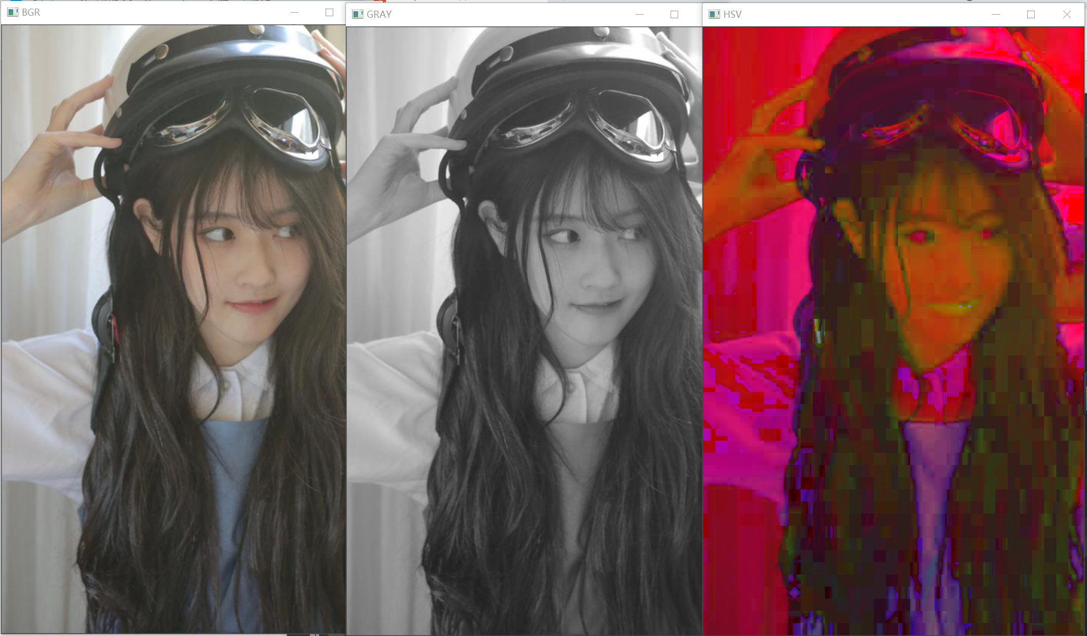
There are more than 150 color space conversion methods in OpenCV. However, we only need to study the two most commonly used methods: BGR to GRAY and BGR to HSV.

We use the cv.cvtColor(input_image, flag) function for color conversion, where flag determines the type of conversion.

For BGR to Gray conversion, we set the flag to cv2.COLOR_BGR2GRAY. Similarly, for BGR to HSV, we set the flag to cv2.COLOR_BGR2HSV.

code:

import cv2

BGR = cv2.imread("C:/Users/Zhang-Lei/Desktop/snack.png")
GRAY = cv2.cvtColor(BGR, cv2.COLOR_BGR2GRAY)
HSV = cv2.cvtColor(BGR, cv2.COLOR_BGR2HSV)

cv2.imshow('BGR', BGR)
cv2.imshow('GRAY', GRAY)
cv2.imshow('HSV', HSV)
cv2.resizeWindow('BGR', 500, 800)
cv2.resizeWindow('GRAY', 500, 800)
cv2.resizeWindow('HSV', 500, 800)
cv2.waitKey()
cv2.destroyAllWindows()

result:

To get other flag values, we just need to enter the code to view:

code:

flags = [i for i in dir(cv2) if i.startswith('COLOR_')]
print(flags)

There are too many kinds, so we won't show the results here.

Note: for HSV, hue range is [0179], saturation range is [0255], and brightness value is [0255]. Different software uses different proportions. Therefore, if you want to compare the value of OpenCV with that of other software, you need to normalize these ranges.

Target tracking

Now that we know how to convert BGR images into HSV images, we can use it to extract color objects. HSV is easier to represent color in color space than BGR. In our application, we will try to extract a blue color object by:

1. Extract each video frame.
2. Convert BGR to HSV color space.
3. We threshold the HSV image with the range of blue pixels.
4. Now that we have extracted the blue object, we can deal with the picture at will.

code:

import cv2
import numpy as np

cap = cv2.VideoCapture(0)  # Read camera image
while 1:
    _, frame = cap.read()
    hsv = cv2.cvtColor(frame, cv2.COLOR_BGR2HSV)  # Convert to HSV diagram
    lower_blue = np.array([110, 50, 50])  # Limit the lower limit of the blue range
    upper_blue = np.array([130, 255, 255])  # Limit the upper limit of the blue range
    mask = cv2.inRange(hsv, lower_blue, upper_blue)  # Limit HSV image range
    res = cv2.bitwise_and(frame, frame, mask=mask)  # Bitwise AND
    cv2.imshow('frame', frame)
    cv2.imshow('mask', mask)
    cv2.imshow('res', res)
    k = cv2.waitKey(5) & 0xFF  # Detect whether Esc reference &0xff is pressed,
    # It is to take only the last 8 bits of the ASCII value corresponding to the key to eliminate the interference of different keys and judge what the key is.
    if k == 27:
        break
cv2.destroyAllWindows()

result:

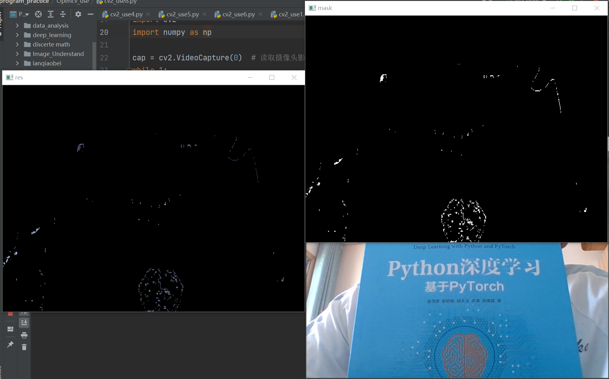
We can see that the blue object of the book has been extracted by us.

How to find the HSV value of a color

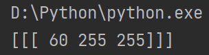
You can use the same function: cv2.cvtColor(). You don't need to enter a picture, you just need to enter the BGR value you need. For example, in order to find the green HSV value,

code:

green = np.uint8([[[0, 255, 0]]])
hsv_green = cv2.cvtColor(green, cv2.COLOR_BGR2HSV)
print(hsv_green)

result:

Graphic transformation

Zoom (cv2.resize())

Zoom is to resize the picture. OpenCV uses the cv2.resize() function to adjust. You can specify the size of the image manually or you can specify a scale factor. Different interpolation methods can be used. For downsampling (image downscaling), the most appropriate interpolation method is cv2.INTER_AREA for up sampling (amplification), the best method is cv2.INTER_CUBIC (slower) and cv2.INTER_LINEAR (faster). By default, the interpolation method used is cv2.INTER_AREA . You can resize the input picture using the following methods:

code:

import cv2

img = cv2.imread("C:/Users/Zhang-Lei/Desktop/snack.png")
res1 = cv2.resize(img, None, fx=1/2, fy=1/2, interpolation=cv2.INTER_CUBIC) # fx and fy correspond to the image magnification of the horizontal and vertical axes respectively

height, width = img.shape[:2]
res2 = cv2.resize(img, (width//2, height//2), interpolation=cv2.INTER_CUBIC) # second method

cv2.imshow('img', img)
cv2.imshow('res1', res1)
cv2.imshow('res2', res2)
cv2.waitKey()
cv2.destroyAllWindows()

result:

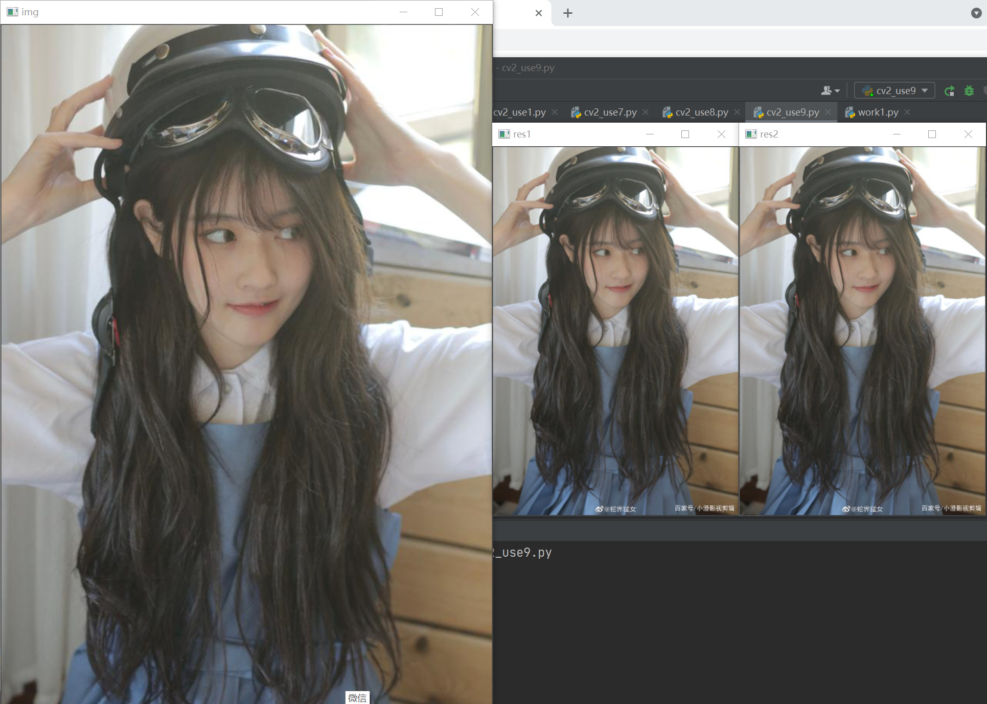
It can be seen that both methods reduce the size of the image to half the original size.

translation

Translation transformation is the movement of the position of an object. If you know the offset in the (x, y) direction, assuming (t_x,t_y), you can create the following conversion matrix M:

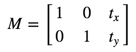
You can save the transformation matrix as a numpy array of type np.float32 and use it as the second parameter of cv.warpAffine. See the following example of conversion (100,50):

code:

import cv2
import numpy as np

img = cv2.imread('C:/Users/Zhang-Lei/Desktop/snack_gray.png', cv2.IMREAD_UNCHANGED)
rows, cols = img.shape
M = np.float32([[1, 0, 100], [0, 1, 50]])
res = cv2.warpAffine(img, M, (cols, rows))
cv2.imshow('img', img)
cv2.imshow('res', res)
cv2.waitKey()
cv2.destroyAllWindows()

result:

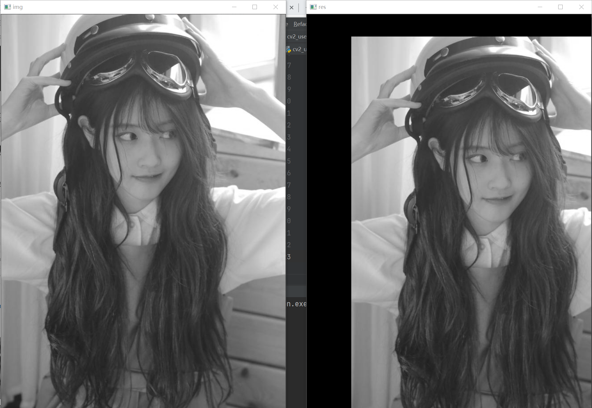
Here you can see that the obtained image is shifted to the lower right compared with the original image.

Note: the third parameter of cv2.warpAffine function is the size of the output image. Its form should be (width, height). Remember that width = number of columns and height = number of rows.

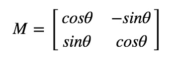
rotate

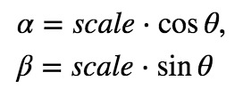
with θ The conversion matrix form of angle rotation picture is:

However, Opencv provides the scale transformation of variable rotation center, so you can rotate the picture at any position. The modified transformation matrix is:

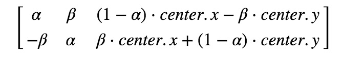
Of which:

To find this transformation matrix, opencv provides a function
cv2.getRotationMatrix2D .
Look at the example below, which rotates the image 90 degrees relative to the center without any scaling.

code:

import cv2

img = cv2.imread('C:/Users/Zhang-Lei/Desktop/snack_gray.png', cv2.IMREAD_UNCHANGED)
rows, cols = img.shape
M = cv2.getRotationMatrix2D(((cols-1)/2.0, (rows-1)/2.0), 90, 1)
res = cv2.warpAffine(img, M, (cols, rows))
cv2.imshow('img', img)
cv2.imshow('res', res)
cv2.waitKey()
cv2.destroyAllWindows()

result:

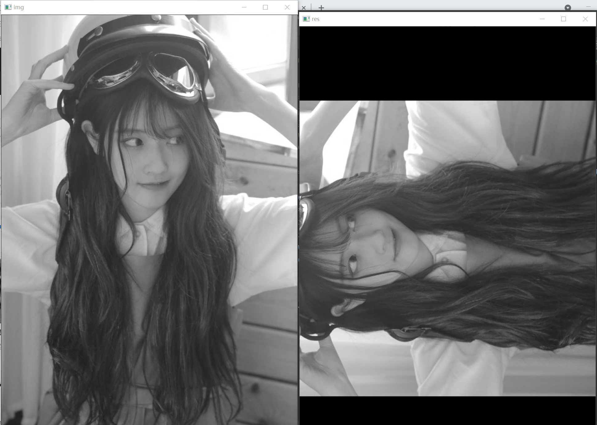
It can be seen that the picture has rotated 90 ° counterclockwise.

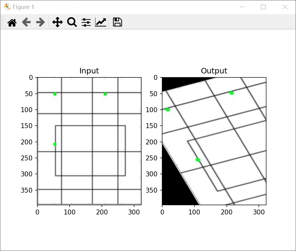
affine transformation

In affine transformation, all parallel lines in the original image are still parallel in the output image. In order to find the transformation matrix, we need to take three points from the input image and their corresponding positions in the output image. Then cv2.getPerspectiveTransform will create a 2x3 matrix, which will be passed to cv2.warpAffine.

code:

import cv2
import matplotlib.pyplot as plt
import numpy as np

img = cv2.imread('C:/Users/Zhang-Lei/Desktop/drawing.png')
rows, cols, ch = img.shape
pts1 = np.float32([[50, 50], [200, 50], [50, 200]])
pts2 = np.float32([[10, 100], [200, 50], [100, 250]])
M = cv2.getAffineTransform(pts1, pts2)
dst = cv2.warpAffine(img, M, (cols, rows))
plt.subplot(121), plt.imshow(img), plt.title('Input')
plt.subplot(122), plt.imshow(dst), plt.title('Output')
plt.show()

result:

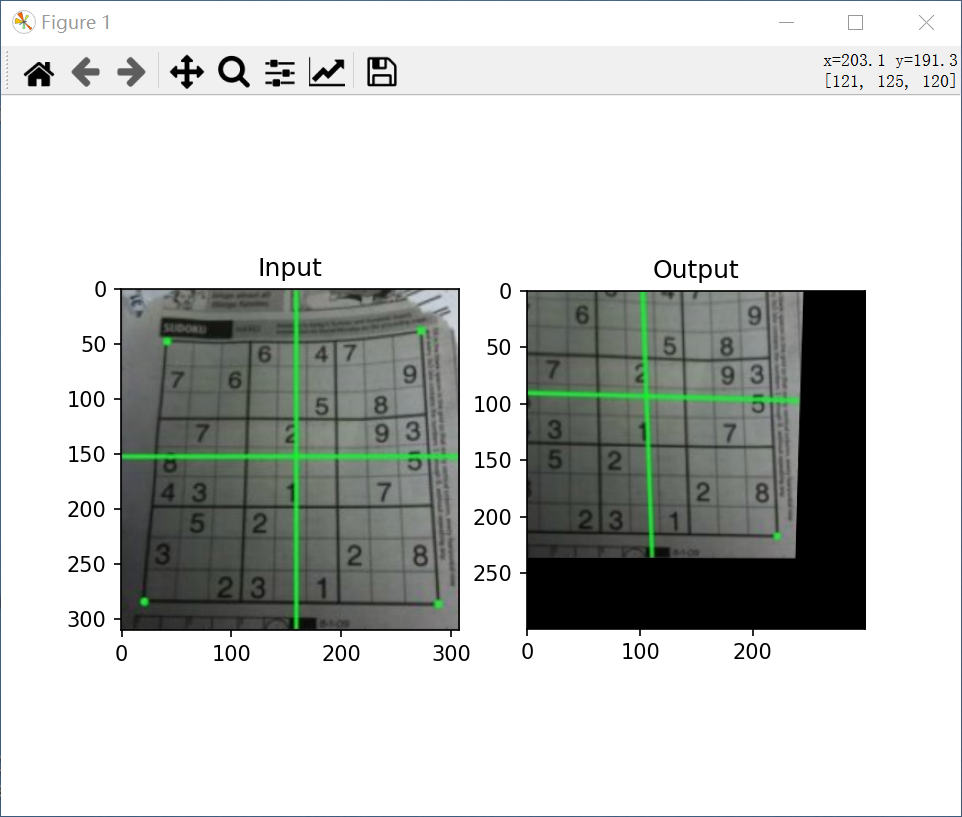
Perspective transformation

For perspective transformation, you need a 3x3 transformation matrix. The line remains straight even after conversion. To find this transformation matrix, you need four points on the input image and the corresponding points on the output image. Among these four points, any three points should not be collinear. Then find the transformation matrix through cv2.getperspective transform. Then use cv2.warpPerspective for this 3x3 transformation matrix.

code:

import cv2
import matplotlib.pyplot as plt
import numpy as np

img = cv2.imread('C:/Users/Zhang-Lei/Desktop/sudoku.png')
rows, cols, ch = img.shape
pts1 = np.float32([[56, 65], [368, 52], [28, 387], [389, 390]])
pts2 = np.float32([[0, 0], [300, 0], [0, 300], [300, 300]])
M = cv2.getPerspectiveTransform(pts1, pts2)
dst = cv2.warpPerspective(img, M, (300, 300))
plt.subplot(121), plt.imshow(img), plt.title('Input')
plt.subplot(122), plt.imshow(dst), plt.title('Output')
plt.show()

result:

Binarization

Simple threshold method

This method is straightforward. If the pixel value is greater than the threshold, it is assigned to one value (possibly white), otherwise it is assigned to another value (possibly black). The function used is cv2.threshold. The first parameter is the source image, which should be a grayscale image. The second parameter is the threshold, which is used to classify pixel values. The third parameter is maxval, which represents the value to be given when the pixel value is greater than (sometimes less than) the threshold. opencv provides different types of thresholds, which are determined by the fourth parameter of the function. Different types are:

• cv.THRESH_BINARY
• cv.THRESH_BINARY_INV
• cv.THRESH_TRUNC
• cv.THRESH_TOZERO
• cv.THRESH_TOZERO_INV

Get two outputs. The first is retval, which will be explained later. The second output is our threshold image.

code:

import cv2
import matplotlib.pyplot as plt

img = cv2.imread('C:/Users/Zhang-Lei/Desktop/snack_gray.png', cv2.IMREAD_UNCHANGED)
ret1, thresh1 = cv2.threshold(img, 127, 255, cv2.THRESH_BINARY)
ret2, thresh2 = cv2.threshold(img, 127, 255, cv2.THRESH_BINARY_INV)
ret3, thresh3 = cv2.threshold(img, 127, 255, cv2.THRESH_TRUNC)
ret4, thresh4 = cv2.threshold(img, 127, 255, cv2.THRESH_TOZERO)
ret5, thresh5 = cv2.threshold(img, 127, 255, cv2.THRESH_TOZERO_INV)
titles = ['Original', 'BINARY', 'BINARY_INV', 'TRUNC', 'TOZERO', 'TOZERO_INV']
images = [img, thresh1, thresh2, thresh3, thresh4, thresh5]
for i in range(6):
    plt.subplot(2, 3, i+1)
    plt.imshow(images[i], cmap='gray')
    plt.title(titles[i])
    plt.xticks([])
    plt.yticks([])
plt.show()

result:

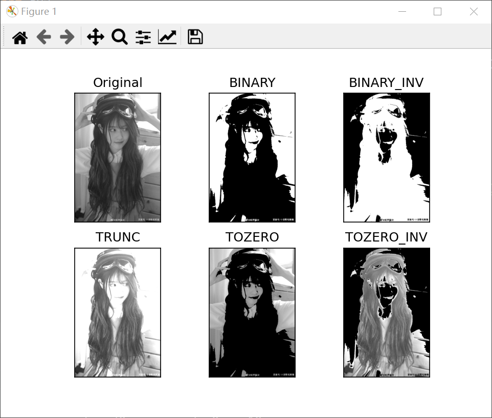
As you can see, the other five images distinguish pixels in different ways.

Adaptive threshold

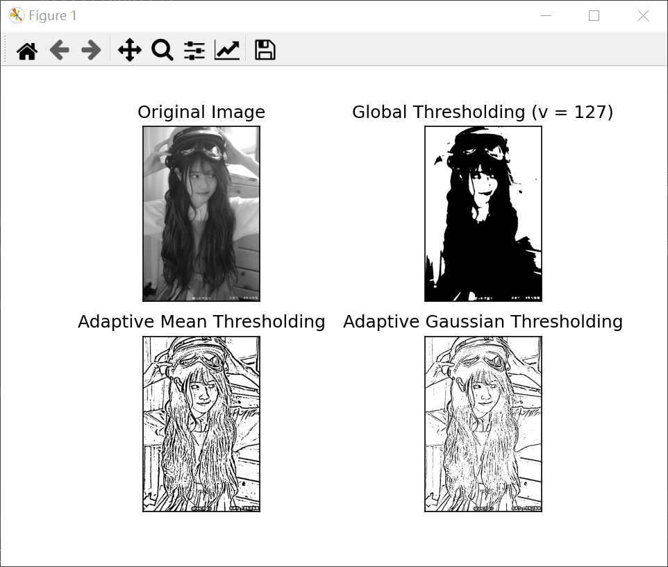
In the previous section, we used a global variable as the threshold. However, this may not be good when the image has different lighting conditions in different areas. In this case, we use adaptive threshold. Here, the algorithm calculates the threshold of a small region of the image. Therefore, we get different thresholds for different regions of the same image, and get better results for images under different illumination.

It has three "special" input parameters and only one output parameter.

• Adaptive Method: it determines how the threshold is calculated.

• cv2.ADAPTIVE_THRESH_MEAN_C: Threshold refers to the average value of adjacent areas.

• cv2.ADAPTIVE_THRESH_GAUSSIAN_C: The threshold value is the weighted sum of neighborhood values whose weight is Gaussian window.

• Block Size: it determines the size of the window area where the threshold is calculated.

• C: It is just a constant that is subtracted from the average or weighted average.

The following code compares the global threshold and adaptive threshold of images with different illumination:

code:

import cv2
import matplotlib.pyplot as plt

img = cv2.imread('C:/Users/Zhang-Lei/Desktop/snack_gray.png', 0)
img = cv2.medianBlur(img, 5)
ret, thresh1 = cv2.threshold(img, 127, 255, cv2.THRESH_BINARY)
thresh2 = cv2.adaptiveThreshold(img, 255, cv2.ADAPTIVE_THRESH_MEAN_C,cv2.THRESH_BINARY, 11, 2)
thresh3 = cv2.adaptiveThreshold(img, 255, cv2.ADAPTIVE_THRESH_GAUSSIAN_C,cv2.THRESH_BINARY, 11, 2)
titles = ['Original Image', 'Global Thresholding (v = 127)',
          'Adaptive Mean Thresholding', 'Adaptive Gaussian Thresholding']
images = [img, thresh1, thresh2, thresh3]
for i in range(4):
    plt.subplot(2, 2, i + 1), plt.imshow(images[i], 'gray')
    plt.title(titles[i])
    plt.xticks([]), plt.yticks([])
plt.show()

result:

Otsu binarization (commonly known as Otsu method)

In the first part, there is a parameter retval. When we binarize Otsu, its purpose comes. What's that?

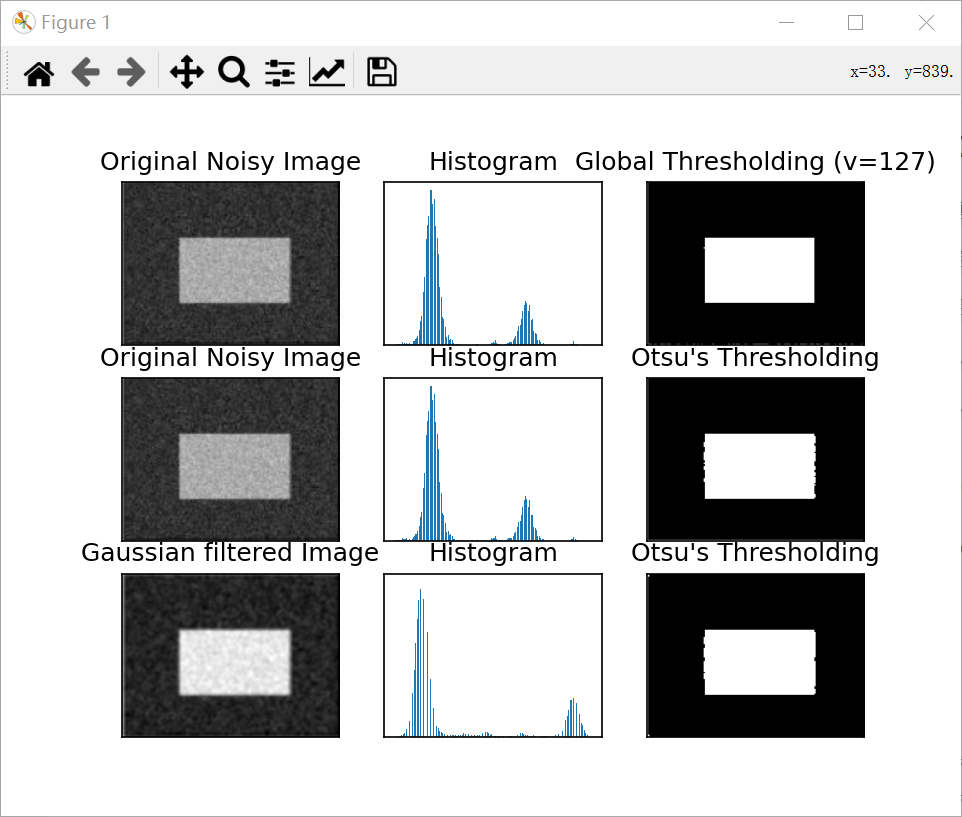
In global thresholding, we use an arbitrary threshold, right? So how do we know whether the value we choose is good or bad? The answer is trial and error. But consider a bimodal image (in short, a bimodal image is an image with two peaks in a histogram). For that image, we can approximately take one of these peaks as the threshold, right? This is what Otsu binarization does. So simply put, it will automatically calculate the threshold from the image histogram of the bimodal image. (for non bimodal images, binarization will not be accurate.)

To do this, we used the cv2.threshold function, but passed an additional symbol cv2.threshold_ otsu . For the threshold, just pass in zero. Then, the algorithm finds the optimal threshold and returns retval as the second output. If you do not use the otsu threshold, the retval is the same as the threshold you use.

See the example below. The input image is a noise image. In the first case, I applied a global threshold value of 127. In the second case, I apply the otsu threshold directly. In the third case, I use 5x5 Gaussian kernel to filter the image to remove noise, and then apply otsu threshold. See how noise filtering improves results.

code:

import cv2
import matplotlib.pyplot as plt

img = cv2.imread('C:/Users/Zhang-Lei/Desktop/noisy.png', 0)
# Global threshold
ret1, thresh1 = cv2.threshold(img, 127, 255, cv2.THRESH_BINARY)
# Otsu threshold
ret2, thresh2 = cv2.threshold(img, 0, 255, cv2.THRESH_BINARY + cv2.THRESH_OTSU)
# Otsu threshold after Gaussian filtering
blur = cv2.GaussianBlur(img, (5, 5), 0)
ret3, thresh3 = cv2.threshold(blur, 0, 255, cv2.THRESH_BINARY + cv2.THRESH_OTSU)
# Draw all the images and their histograms
images = [img, 0, thresh1, img, 0, thresh2, blur, 0, thresh3]
titles = ['Original Noisy Image', 'Histogram', 'Global Thresholding (v=127)',
          'Original Noisy Image', 'Histogram', "Otsu's Thresholding",
          'Gaussian filtered Image', 'Histogram', "Otsu's Thresholding"]
for i in range(3):
    plt.subplot(3, 3, i * 3 + 1), plt.imshow(images[i * 3], 'gray')
    plt.title(titles[i * 3]), plt.xticks([]), plt.yticks([])
    plt.subplot(3, 3, i * 3 + 2), plt.hist(images[i * 3].ravel(), 256)
    plt.title(titles[i * 3 + 1]), plt.xticks([]), plt.yticks([])
    plt.subplot(3, 3, i * 3 + 3), plt.imshow(images[i * 3 + 2], 'gray')
    plt.title(titles[i * 3 + 2]), plt.xticks([]), plt.yticks([])
plt.show()

result:

Otsu binarization principle

This section demonstrates the python implementation of otsu binarization to show how it actually works.

Since we use a bimodal image, Otsu's algorithm attempts to find a threshold (t), which minimizes the weighted variance within the class calculated by the following formula:

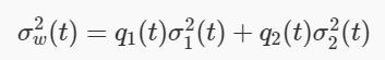
Of which:

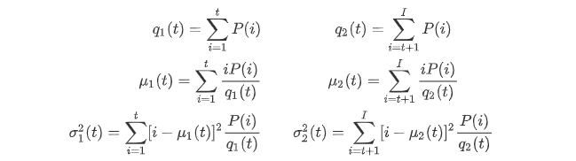
It actually finds a T value, which lies between the two peaks, minimizing the variance of the two classes. It can be simply implemented in python as follows:

code:

import cv2
import numpy as np

img = cv2.imread('C:/Users/Zhang-Lei/Desktop/noisy.png', 0)
blur = cv2.GaussianBlur(img, (5, 5), 0)
# Find the normalized histogram and the cumulative distribution function
hist = cv2.calcHist([blur], [0], None, [256], [0, 256])
hist_norm = hist.ravel() / hist.max()
Q = hist_norm.cumsum()
bins = np.arange(256)
fn_min = np.inf
thresh = -1
for i in range(1, 256):
    p1, p2 = np.hsplit(hist_norm, [i])  # probability
    q1, q2 = Q[i], Q[255] - Q[i]  # Category sum
    b1, b2 = np.hsplit(bins, [i])  # weight
    # f find the mean and variance
    m1, m2 = np.sum(p1 * b1) / q1, np.sum(p2 * b2) / q2
    v1, v2 = np.sum(((b1 - m1) ** 2) * p1) / q1, np.sum(((b2 - m2) ** 2) * p2) / q2
    # Calculate minimum function
    fn = v1 * q1 + v2 * q2
    if fn < fn_min:
        fn_min = fn
        thresh = i
# otsu 'threshold with Opencv2 function
ret, otsu = cv2.threshold(blur, 0, 255, cv2.THRESH_BINARY + cv2.THRESH_OTSU)
print("{} {}".format(thresh, ret))

result:

wave filtering

Two dimensional convolution (image filtering)

Like one-dimensional signals, images can also be filtered by various low-pass filters (LPF), high pass filters (HPF), etc. LPF helps eliminate noise, blurred images, etc. The HPF filter helps to find edges in the image.

opencv provides the function cv2.filter2D(), which is used to convolute the kernel with the image. As an example, we will try to perform mean filtering on the image. The 5x5 mean filter convolution kernel is as follows:

The operation is as follows: align the center of the kernel with a pixel, then add all 25 pixels under the kernel, take the average value, and replace the center pixel of the 25x25 window with the new average value. It continues to do this for all pixels in the image. Try the following code and observe the result:

code:

import cv2
import numpy as np
from matplotlib import pyplot as plt

img = cv2.imread('C:/Users/Zhang-Lei/Desktop/noisy.png')
kernel = np.ones((5, 5), np.float32) / 25
dst = cv2.filter2D(img, -1, kernel)
plt.subplot(121), plt.imshow(img), plt.title('Original')
plt.xticks([]), plt.yticks([])
plt.subplot(122), plt.imshow(dst), plt.title('Averaging')
plt.xticks([]), plt.yticks([])
plt.show()

result:

It can be seen that the image becomes blurred under the action of filtering.

Image blur (image smoothing)

Image blur is realized by convoluting the image with low-pass filter kernel. It helps to eliminate noise. It actually removes high-frequency content (e.g. noise, edges) from the image. So in this operation, the edge is a little fuzzy. Well, there are some blur techniques that don't blur the edges too much. OpenCV mainly provides four fuzzy technologies.

Mean filtering

This is accomplished by convoluting the image with a normalized filter core. It simply takes the average of all pixels under the kernel area and replaces the central element. This is done through the functions cv2.blur() or cv2.boxFilter(). For more details about the kernel, see the documentation. We should specify the width and height of the filter core. The 3x3 standardized frame filter is as follows:

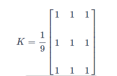
Note: if you do not use standardized filtering, use cv2.boxFilter() to pass in the parameter normalize=False.

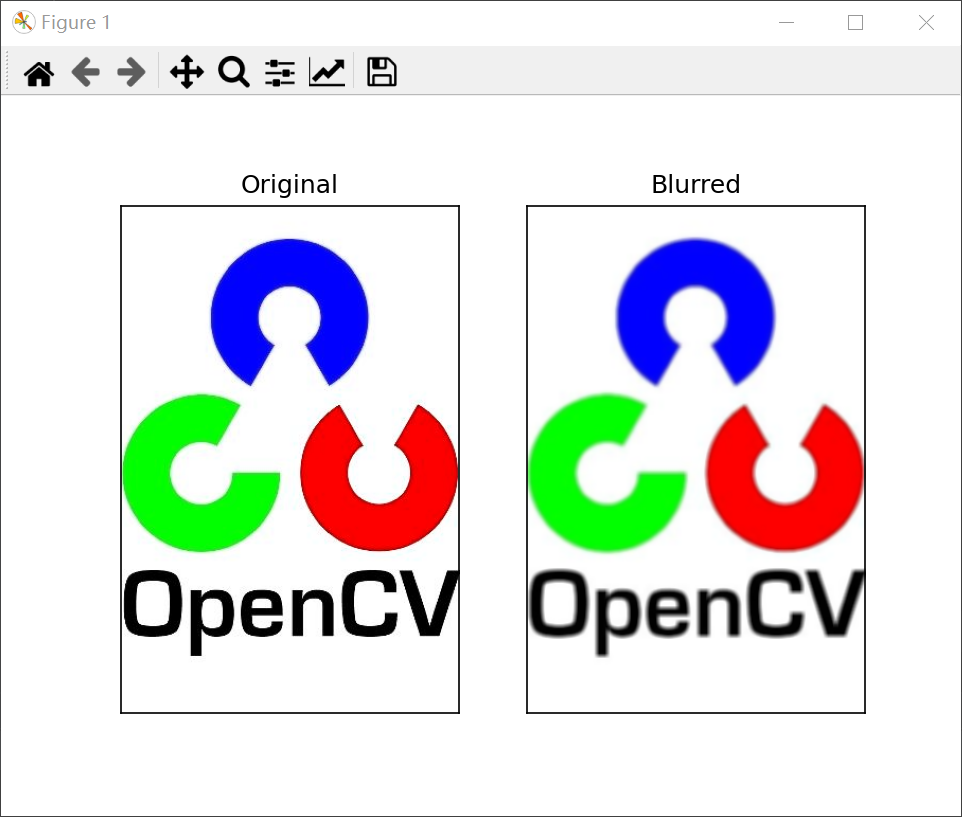
The simple application of 5x5 core is as follows:

import cv2
from matplotlib import pyplot as plt

img = cv2.imread('C:/Users/Zhang-Lei/Desktop/opencv.jpg')
blur = cv2.blur(img, (5, 5))
plt.subplot(121), plt.imshow(img), plt.title('Original')
plt.xticks([]), plt.yticks([])
plt.subplot(122), plt.imshow(blur), plt.title('Blurred')
plt.xticks([]), plt.yticks([])
plt.show()

result:

Gaussian filtering

In this case, Gaussian kernel is used instead of kernel filter. It is done through the function * * CV2. Gaussian blur() *. We should specify the width and height of the kernel. It should be positive and odd (odd has a median). We should also specify the standard deviation, sigmax and sigmay in the x and y directions, respectively. If only sigmax is specified, sigmay is the same as sigmax. If both values are 0, they are calculated based on the kernel size. Gaussian blur is an effective method to eliminate Gaussian noise in image.

If necessary, you can create a Gaussian kernel using the function cv. Getgaussian kernel().

The above code can be modified as Gaussian filter:

blur = cv2.GaussianBlur(img,(5,5),0)

code:

import cv2
from matplotlib import pyplot as plt

img = cv2.imread('C:/Users/Zhang-Lei/Desktop/opencv.jpg')
blur = cv2.GaussianBlur(img, (5, 5), 0)
plt.subplot(121), plt.imshow(img), plt.title('Original')
plt.xticks([]), plt.yticks([])
plt.subplot(122), plt.imshow(blur), plt.title('GaussianBlurred')
plt.xticks([]), plt.yticks([])
plt.show()

result:

median filtering

Here, the function cv2.medianBlur() takes the median value of all pixels under the kernel area and replaces the central element with the median value. This is very effective for salt and pepper noise in the image. Interestingly, in the above filter, the central element is a newly calculated value, which may be a pixel value in the image or a new value. However, in median blur, the central element is always replaced by some pixel values in the image, which can effectively reduce the noise. Its kernel size should be a positive odd integer.

In this demonstration, I added 5000 salt and pepper noises to the original image and applied intermediate blur. Just change the above code to median filter:

median = cv2.medianBlur(img,5)

code:

import random
import cv2
from matplotlib import pyplot as plt


# Add salt and pepper noise
def noise(dst):
    height, width = dst.shape[:2]
    for _ in range(height*width//4):
        x = random.randint(0, height-1)
        y = random.randint(0, width-1)
        dst[x, y] = 255  # Add salt noise
        p = random.randint(0, height-1)
        q = random.randint(0, width-1)
        dst[p, q] = 0  # Add pepper noise


img = cv2.imread('C:/Users/Zhang-Lei/Desktop/snack_gray.png', 0)
plt.subplot(131), plt.imshow(img, cmap='gray'), plt.title('Original')
plt.xticks([]), plt.yticks([])
noise(img)
plt.subplot(132), plt.imshow(img, cmap='gray'), plt.title('Noise')
plt.xticks([]), plt.yticks([])
median = cv2.medianBlur(img, 5)
plt.subplot(133), plt.imshow(median, cmap='gray'), plt.title('MedianBlurred')
plt.xticks([]), plt.yticks([])
plt.show()

result:

It can be seen that the second picture adds noise on the basis of the original picture. Although the third picture removes the noise, it will still be partially blurred.

Bilateral filtering

CV2. Bilaterfilter () is very effective for noise removal while maintaining sharp edges. However, compared with other filters, the operation speed is slower. We have seen that the Gaussian filter takes the neighborhood around the pixel and finds its Gaussian weighted average. The Gaussian filter is a spatial function, that is, adjacent pixels are considered in filtering. However, it does not consider whether the pixel has almost the same intensity or whether the pixel is an edge pixel. So it also blurs the edges, which we don't want to do.

The bilateral filter also adopts Gaussian filter in space, and the other Gaussian filter is a function of pixel difference. The Gaussian function of space ensures that the blur only considers adjacent pixels, while the Gaussian function of intensity difference ensures that the blur only considers pixels with similar intensity to the central pixel. So it preserves the edge, because the pixels at the edge will have a great change in intensity.

The following example shows the use of bilateral filter. Similarly, you only need to change the above code to bilateral filter:

blur = cv2.bilateralFilter(img,9,75,75)

code:

import cv2
from matplotlib import pyplot as plt

img = cv2.imread('C:/Users/Zhang-Lei/Desktop/snack_gray.png', 0)
plt.subplot(121), plt.imshow(img, cmap='gray'), plt.title('Original')
plt.xticks([]), plt.yticks([])
blur = cv2.bilateralFilter(img, 9, 75, 75)
plt.subplot(122), plt.imshow(blur, cmap='gray'), plt.title('BilateralBlurred')
plt.xticks([]), plt.yticks([])
plt.show()

result:

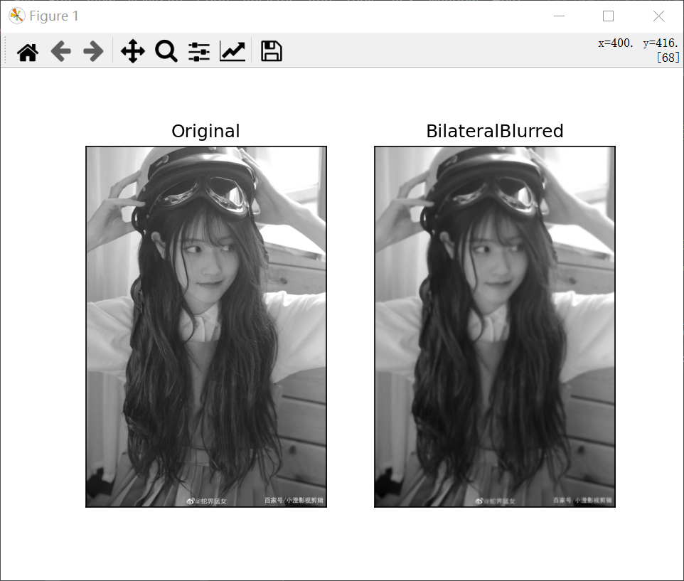
The visible image becomes blurred after bilateral filtering.