1 Introduction to algorithm

1.1 introduction to the principle of BP neural network

Neural network is the basis of deep learning. It is widely used in machine learning and deep learning, such as function approximation, pattern recognition, classification model, image classification, CTR prediction based on deep learning, data compression, data mining and so on. The following mainly introduces the principle of BP neural network.

The simplest three-layer BP neural network is shown in the figure below

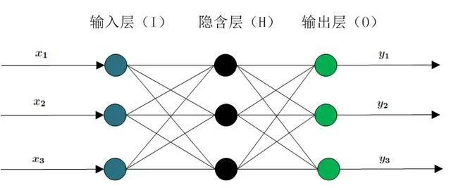
It includes input layer, hidden layer and output layer, and there are weights between nodes. A sample has m input features, including ID features or continuous features. There can be multiple hidden layers. The selection of the number of hidden layer nodes is generally set to the nth power of 2, such as 512256128, 64, 32, etc. n output results, usually one output result, such as classification model or regression model.

In 1989, Robert Hecht Nielsen proved that a continuous function in any closed interval can be approximated by a hidden layer BP network, which is the universal approximation theorem. Therefore, a three-layer BP network can complete any m-dimensional to n-dimensional mapping. BP neural network is mainly divided into two processes

1. Working signal forward transfer subprocess

2. Error signal reverse transfer subprocess

1 working signal forward transmission subprocess

Let the weight between node i and node j be ω {ij}, the offset of node j is b{j}, and the output value of each node is x_{j} , the output value of each node is calculated according to the output value of all nodes in the upper layer, the weight of the current node and all nodes in the upper layer, the offset of the current node and the activation function. The specific calculation formula is as follows:

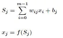
Where f is the activation function, S-type function or tanh function is generally selected. The forward transfer process is relatively simple, which can be calculated from front to back.

2 error signal reverse transmission subprocess

In BP neural network, the sub process of error signal reverse transmission is complex, which is based on Widrow Hoff learning rule. Assume that all results of the output layer are d_{j} , the error function of the regression model is as follows

The main purpose of BP neural network is to repeatedly modify the weight and bias to minimize the value of error function. Widrow Hoff learning rule is to continuously adjust the weight and bias of the network along the steepest descent direction of the sum of squares of relative errors. According to the gradient descent method, the correction of the weight vector is directly proportional to the gradient of E(w,b) at the current position, and it is effective for the j-th output node

Suppose the selected activation function is

The derivation of the activation function is obtained

So next for ω_ {ij}, yes

among

Also for b_{j} , yes

This is the famous δ Learning rules reduce the error between the actual output and expected output of the system by changing the connection weight between neurons. This rule is also called Widrow Hoff learning rules or error correction learning rules.

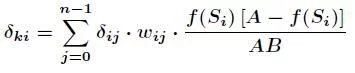
The above is to calculate the adjustment amount for the weight between the hidden layer and the output layer and the offset of the output layer, while the calculation of the offset adjustment amount for the input layer, the hidden layer and the hidden layer is more complex. hypothesis ω_ {ki} is the weight between the k-th node of the input layer and the i-th node of the hidden layer

Among them

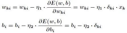
With the above formula, according to the gradient descent method, the weight and offset between the hidden layer and the output layer are adjusted as follows

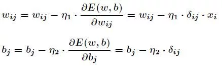
The adjustment of weight and offset between input layer and hidden layer is also important

The above is the formula derivation of the principle of BP neural network.

  1.3 differential evolution algorithm

Differential Evolution(DE) was proposed by Storn et al. In 1995, and others Evolutionary algorithm Similarly, DE is a simulation of biological evolution stochastic model , through repetition iteration , so that those individuals who adapt to the environment are preserved. However, compared with evolutionary algorithm, DE retains the global search strategy based on population, and adopts real number coding, simple mutation operation based on difference and one-to-one competitive survival strategy to reduce the complexity of genetic operation. At the same time, the unique memory ability of DE enables it to dynamically track the current search situation to adjust its search strategy, and has strong global convergence and stability Robustness It is suitable for solving some optimization problems in complex environment that can not be solved by conventional mathematical programming methods. At present, DE has been applied in many fields, such as manual neuron Network, chemical industry, electric power, mechanical design, robot, signal processing, biological information, economics, modern agriculture, food safety, environmental protection and operations research.

DE algorithm is mainly used to solve continuous variable The main working steps of the global optimization problem are the same as others evolutionary algorithms Basically consistent, mainly including mutation, crossover and selection. The basic idea of the algorithm is to start from a randomly generated initial population, use the difference vector of two individuals randomly selected from the population as the random change source of the third individual, weigh the difference vector and sum it with the third individual according to certain rules to generate a mutated individual. This operation is called mutation. Then, the variant individual is mixed with a predetermined target individual to generate the test individual. This process is called crossover. If the fitness value of the test individual is better than that of the target individual, the test individual will replace the target individual in the next generation, otherwise the target individual will still be saved. This operation is called selection. In the evolution process of each generation, each individual vector is used as the target individual once. Through continuous iterative calculation, the algorithm retains good individuals, eliminates poor individuals, and guides the search process to the global Optimal solution approach.

Algorithm diagram:

Algorithm pseudocode:

Part 2 code

%% Application of differential evolution algorithm to optimization BP Initial weights and thresholds of neural networks

%% Clear environment variables
clear all;
clc;
warning off
load v357;
load y357;
Pn_train=v;
Tn_train=y;
Pn_test=v;
Tn_test=y;
P_train=v;
 T_train=y;
% P_train=[0 25.27 44 62.72 81.4 100.2;
%     290.5 268.8 247.2 224.5 206 184.4;
%     0 16.12 33.25 50.42 67.62 84.73;
%     542.5 517.8 493 465.3 435.6 410.8;
%     0 11.1 28.1 44.93 61.38 78.57;
%     826.1 800.2 769.1 740.0 706.2 669.3];
% T_train=[0 1 2 3 4 5];%These are unprocessed data
%  P_test=[0 25.25 43 62.75 81.6 100.7;
%     290.3 268.4 247.5 224.6 206 184.2;
%     0 16.14 33.26 50.47 67.68 84.79;
%     542.7 517.9 495 465.8 435.6 410.9;
%     0 11.4 28.6 44.94 61.36 78.59;
%     826.3 800.7 769.8 740.5 706.7 669.3];
% T_test=[0 1 2 3 4 5];

% Pn_train=[0 0.252 0.439 0.626 0.813 1 0 0.19 0.392 0.595 0.798 1 0 0.141 0.358 0.572 0.781 1;
%           1 0.795 0.592 0.378 0.204 0 1 0.815 0.626 0.415 0.189 0 1 0.835 0.637 0.451 0.235 0];
% %T Is the target vector, normalized data
% Tn_train=[0.05,0.23,0.41,0.59,0.77,0.95,0.05,0.23,0.41,0.59,0.77,0.95,0.05,0.23,0.41,0.59,0.77,0.95]; 
% Pn_test=[ 0 0.17 0.39 0.595 0.798 1 0 0.141 0.358 0.572 0.781 1 0 0.258 0.439 0.626 0.813 1;
%          1 0.815 0.625 0.415 0.189 0 1 0.835 0.635 0.451 0.235 0 1 0.795 0.599 0.378 0.204 0 ];
% Tn_test=[0.05,0.23,0.41,0.59,0.77,0.95,0.05,0.23,0.41,0.59,0.77,0.95,0.05,0.23,0.41,0.59,0.77,0.95];

%% Parameter setting
S1 = size(Pn_train,1);              % Number of neurons in input layer
S2 = 6;                            % Number of hidden layer neurons
S3 = size(Tn_train,1);              % Number of neurons in output layer
Gm=10;    %Maximum number of iterations
F0=0.5;      %F Scale factor
Np=5; %Population size
CR=0.5;  %Hybridization parameters
G=1;%Initialization algebra
N=S1*S2 + S2*S3 + S2 + S3;%Dimension of the problem


% Set the initial weight and threshold of the network
net_optimized.IW{1,1} = W1;
net_optimized.LW{2,1} = W2;
net_optimized.b{1} = B1;
net_optimized.b{2} = B2;
% Set training parameters
net_optimized.trainParam.epochs = 3000;
net_optimized.trainParam.show = 100;
net_optimized.trainParam.goal = 0.001;
net_optimized.trainParam.lr = 0.1;

% The new weights and thresholds are used for training
net_optimized = train(net_optimized,Pn_train,Tn_train);

%% Simulation test
Tn_sim_optimized = sim(net_optimized,Pn_test);     


% Comparison of results
result_optimized = [Tn_test' Tn_sim_optimized'];

%Mean square error
E_optimized = mse(Tn_sim_optimized - Tn_test)
MAPE_optimized = mean(abs(Tn_sim_optimized-Tn_test)./Tn_sim_optimized)*100

% figure(1)
% 
% plot(T_train,P_train(1,:),'r')
% hold on 
% plot(T_train,P_train(3,:),'y')
% hold on
% plot(T_train,P_train(5,:),'b')
% hold on
% grid on
% xlabel('Agreed true value of standard equipment (10) KP)');
%  ylabel('Output of pressure sensor( mv)');
%  title('Working curve of pressure sensor');
%  legend('t=22','t=44','t=70');

 figure(2)
plot(Tn_train(1:6),Pn_train(1,1:6),'r')
hold on 
plot(Tn_train(7:12),Pn_train(1,7:12),'y')
hold on
plot(Tn_train(13:18),Pn_train(1,13:18),'b')
hold on
grid on
xlabel('Agreed true value of equipment (10) KP)');
 ylabel('Output of pressure sensor( mv)');
 title('Normalized training sample pressure sensor working curve');
 legend('t=22','t=44','t=70');
 
 figure(3)
plot(Tn_test(1:6),Pn_test(1,1:6),'r')
hold on 
plot(Tn_test(7:12),Pn_test(1,7:12),'y')
hold on
plot(Tn_test(13:18),Pn_test(1,13:18),'b')
hold on
grid on
xlabel('Agreed true value of equipment (10) KP)');
 ylabel('Output of pressure sensor( mv)');
 title('Normalized test sample pressure sensor working curve');
 legend('t=22','t=44','t=70');
 
 
 figure(4)
plot(Tn_test(1:6),Tn_sim_optimized(1:6),'r')%output DE-BP Curve of simulation results
hold on
 plot(Tn_test(7:12),Tn_sim_optimized(7:12),'y')
 hold on
 plot(Tn_test(13:18),Tn_sim_optimized(13:18),'b')
 hold on
 xlabel('Agreed truth value (10) KP)');
 ylabel('Output of pressure sensor( mv)');
 title('DE-BP Working curve of pressure sensor');
 legend('t=22','t=44','t=70');
grid on








%% Not optimized BP neural network
%net = newff(Pn_train,Tn_train,S2);
net=newff(minmax(Pn_train),[6,1],{'logsig','purelin'},'traingdm');%Hidden layer neuron S Type tangent,Output layer S Type logarithm, momentum gradient descent method, training BP network,
% Set training parameters
net.trainParam.epochs = 3000;
net.trainParam.show = 100;
net.trainParam.goal = 0.001;
net.trainParam.lr = 0.1;

net=init(net);
 
inputWeights=net.IW{1,1};% Current input layer weights and thresholds
inputbias=net.b{1};
layerWeights=net.LW{2,1};% Current network layer weights and thresholds 
layerbias=net.b{2}
% The new weights and thresholds are used for training
net = train(net,Pn_train,Tn_train);

%% Simulation test
Tn_sim = sim(net,Pn_test);    


%% Comparison of results
result = [Tn_test' Tn_sim'];
% Mean square error
E1 = mse(Tn_sim - Tn_test)
MAPE1= mean(abs(Tn_sim-Tn_test)./Tn_sim)*100
% end
% figure(4)
% plot(T_train,P_train(1,:),'r')
% hold on 
% plot(T_train,P_train(3,:),'y')
% hold on
% plot(T_train,P_train(5,:),'b')
% hold on
% grid on
% xlabel('Agreed true value of standard equipment (10) KP)');
%  ylabel('Output of pressure sensor( mv)');
%  title('Working curve of pressure sensor');
%  legend('t=22','t=44','t=70');

 figure(5)
plot(Tn_test(1:6),Tn_sim(1:6),'r')%output BP Curve of simulation results
hold on
 plot(Tn_test(7:12),Tn_sim(7:12),'y')
 hold on
 plot(Tn_test(13:18),Tn_sim(13:18),'b')
 hold on
 xlabel('Agreed truth value (10) KP)');
 ylabel('Output of pressure sensor( mv)');
 title('BP Working curve of pressure sensor');
 legend('t=22','t=44','t=70');
grid on

3 simulation results

4 references

[1] Niu Qing, Cao Aimin, Chen Xiaoyi, Zhou Dong. Short term load forecasting based on flower pollination algorithm and BP neural network [J]. Power grid and clean energy, 2020,36 (10): 28-32