1 Introduction to algorithm
1.1 principle of BP neural network algorithm affected by relevant indexes
As shown in Figure 1, when training BP using MATLAB's newff function, it can be seen that most cases are three-layer neural networks (i.e. input layer, hidden layer and output layer). Here to help understand the principle of neural network:
1) Input layer: equivalent to human facial features. The facial features obtain external information and receive input data corresponding to the input port of neural network model.
2) hidden Layer: corresponding to the human brain, the brain analyzes and thinks about the data transmitted from the five senses. The hidden Layer of neural network maps the data X transmitted from the input layer, which is simply understood as a formula hidden Layer_ output=F(w*x+b). Among them, W and B are called weight and threshold parameters, and F() is the mapping rule, also known as the activation function, hiddenLayer_output is the output value of the hidden Layer for the transmitted data mapping. In other words, the hidden Layer maps the input influencing factor data X and generates the mapping value.
3) Output layer: it can correspond to human limbs. After thinking about the information from the five senses (hidden layer mapping), the brain controls the limbs to perform actions (respond to the outside). Similarly, the output layer of BP neural network is hidden layer_ Output is mapped again, outputLayer_output=w *hiddenLayer_output+b. Where W and B are weight and threshold parameters, and outputLayer_output is the output value (also called simulation value and prediction value) of the output layer of the neural network (understood as the external executive action of the human brain, such as the baby slapping the table).
4) Gradient descent algorithm: by calculating outputlayer_ For the deviation between output and the y value input by the neural network model, the algorithm is used to adjust the weight, threshold and other parameters accordingly. This process can be understood as that the baby beats the table and deviates. Adjust the body according to the distance of deviation, so that the arm waved again keeps approaching the table and finally hits the target.
Take another example to deepen understanding:
The BP neural network shown in Figure 1 has input layer, hidden layer and output layer. How does BP realize the output value outputlayer of the output layer through these three-layer structures_ Output, constantly approaching the given y value, so as to train to obtain an accurate model?
From the serial ports in the figure, we can think of a process: take the subway and imagine Figure 1 as a subway line. One day when Wang went home by subway: he got on the bus at the input starting station, passed many hidden layers on the way, and then found that he had overstepped (outputLayer corresponds to the current position), so Wang will return to the midway subway station (hidden layer) to take the subway again according to the distance (Error) from home (Target) according to the current position (the Error is transferred back, and the gradient descent algorithm is used to update w and b). If Wang makes another mistake, the adjustment process will be carried out again.
From the example of baby slapping the table and Wang taking the subway, think about the problem: for the complete training of BP, you need to first input the data to the input, then map through the hidden layer, and get the BP simulation value from the output layer. Adjust the parameters according to the error between the simulation value and the Target value, so that the simulation value constantly approaches the Target value. For example, (1) the baby is affected by external interference factors (x) In response, the brain constantly adjusts the position of the arms and controls the accuracy of the limbs (y, Target). (2) Wang goes to the boarding point (x), crosses the station (predict), and constantly returns to the midway station to adjust the position and get home (y, Target).
In these links, the influencing factor data x and the Target value data y (Target) are involved According to x and y, BP algorithm is used to find the law between x and y, and realize the mapping and approximation of Y by x. This is the role of BP neural network algorithm. In addition, the above process is BP model training, so although the training of the final model is accurate, the law is found (bp network) Whether it is accurate and reliable. Therefore, we give x1 to the trained bp network to obtain the corresponding BP output value (predicted value) Predict1, by mapping and calculating Mse, Mape, R and other indicators to compare the proximity of predict1 and y1, we can know whether the prediction of the model is accurate. This is the test process of BP model, that is, to realize the prediction of data, and compare the actual value to test whether the prediction is accurate.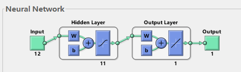
Fig. 1 3-layer BP neural network structure
1.2 BP neural network based on the influence of historical value
Taking the power load forecasting problem as an example, the two models are distinguished. When forecasting the power load in a certain period of time:
One approach is to consider t The climate factor indicators at that time, such as the influence of air humidity x1, temperature x2, holidays x3, etc t This is the model mentioned in 1.1 above.
Another approach is to consider that the change of power load value is related to time. For example, it is considered that the power load value at T-1, t-2 and t-3 is related to the load value at t, that is, it satisfies the formula y(t)=F(y(t-1),y(t-2),y(t-3)). When BP neural network is used to train the model, the influencing factor values input to the neural network are historical load values y (t-1), y (t-2) and Y (t-3) In particular, 3 is called autoregressive order or delay. The target output value given to the neural network is y(t).
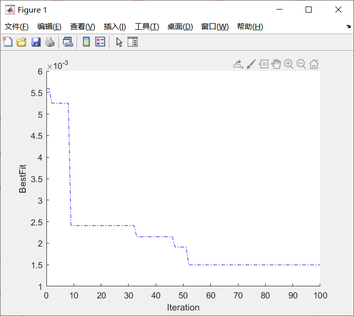
1.3 longicorn whisker algorithm
Algorithm Introduction
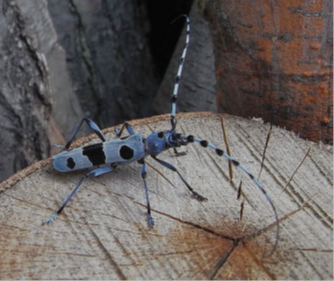
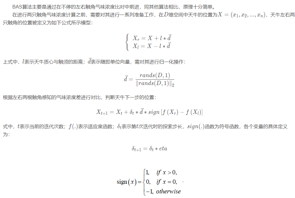
The longicorn beetle whisker search algorithm imitates the foraging behavior of longicorn beetles in nature. During the foraging process of longicorn beetles, food will produce special smell and attract longicorn beetles to move towards food. Longicorn beetles perceive the food smell in the air through their two antennae, and the smell concentration perceived by the two antennae is also different according to the distance between food and the two antennae. When food is in the sky When the cattle is on the left side, the odor concentration perceived by the left antennae is stronger than that perceived by the right antennae. According to the concentration difference perceived by the two antennae, longicorn beetles move randomly towards the side with strong concentration. Through iteration after iteration, they finally find the location of food.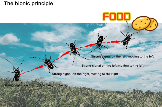
Part 2 code
%% Optimization of search algorithm based on longicorn whisker BP Research on neural network prediction
%% Clear environment variables
clear all
close all
clc
tic
%% Load data
X=xlsread('data.xlsx');
for i=1:111
Y(i)=X(10*(i-1)+1,2);
end
%% Time series data preprocessing
xx = [];
yy = [];
num_input = 3;
tr_len =round(0.8*length(Y));%Number of training set samples
for i = 1:length(Y)-num_input
xx = [xx; Y(i:i+num_input-1)];
yy = [yy; Y(i+num_input)];
end
%BP Input and output of training set
input_train = xx(1:tr_len, :)';
output_train = yy(1:tr_len)';
%BP Input and output of test set
input_test = xx(tr_len+1:end, :)';
output_test = yy(tr_len+1:end)';
%% BP Network settings
%Number of nodes
[inputnum,N]=size(input_train);%Enter the number of nodes
outputnum=size(output_train,1);%Number of output nodes
hiddennum=10; %Hidden layer node
%% data normalization
[inputn,inputps]=mapminmax(input_train,0,1);
[outputn,outputps]=mapminmax(output_train,0,1);% Normalized to[0,1]between
%% Create network
net=newff(inputn,outputn,hiddennum);
net.trainParam.epochs = 1000;
net.trainParam.goal = 1e-3;
% Network output inverse normalization
ABC_sim=mapminmax('reverse',BP_sim,outputps);
% mapping
figure
plot(1:length(output_train),output_train,'b-o','linewidth',1)
hold on
plot(1:length(ABC_sim),ABC_sim,'r-square','linewidth',1)
xlabel('training sample ','FontSize',12);
legend('actual value','Estimate');
axis tight
title('BAS-BP neural network')
% BP Test set
% Normalization of test data
inputn_test=mapminmax('apply',input_test,inputps);
%Prediction output
an=sim(net,inputn_test);
ABCBPsim=mapminmax('reverse',an,outputps);
figure
plot(1:length(output_test), output_test,'b-o','linewidth',1)
hold on
plot(1:length(ABCBPsim),ABCBPsim,'r-square','linewidth',1)
xlabel('Test sample','FontSize',12);
legend('actual value','Estimate');
axis tight
title('BAS-BP neural network')
%% Not optimized BP neural network
net1=newff(inputn,outputn,hiddennum);
% Network evolution parameters
net1.trainParam.epochs=100;
net1.trainParam.lr=0.1;
net1.trainParam.mc = 0.8;%Momentum coefficient,[0 1]between
net1.trainParam.goal=0.001;
% Network training
net1=train(net1,inputn,outputn);
% BP Training set prediction
BP_sim1=sim(net1,inputn);
% Network output inverse normalization
T_sim1=mapminmax('reverse',BP_sim1,outputps);
%Prediction output
an1=sim(net1,inputn_test);
Tsim1=mapminmax('reverse',an1,outputps);
% mapping
figure
plot(1:length(output_train),output_train,'b-o','linewidth',1)
hold on
plot(1:length(T_sim1),T_sim1,'r-square','linewidth',1)
xlabel('training sample ','FontSize',12);
legend('actual value','Estimate');
axis tight
title('BP neural network')
figure
plot(1:length(output_test), output_test,'b-o','linewidth',1)
hold on
plot(1:length(Tsim1),Tsim1,'r-square','linewidth',1)
xlabel('Test sample','FontSize',12);
legend('actual value','Estimate');
axis tight
title('BP neural network')
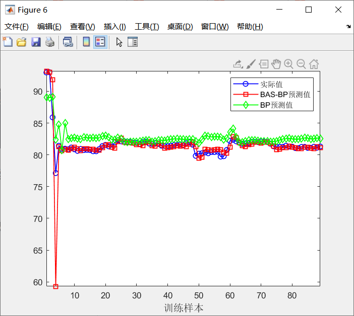
%% ABC-BP and BP Comparison diagram
figure
plot(1:length(output_train),output_train,'b-o','linewidth',1)
hold on
plot(1:length(ABC_sim),ABC_sim,'r-square','linewidth',1)
hold on
plot(1:length(T_sim1),T_sim1,'g-diamond','linewidth',1)
xlabel('training sample ','FontSize',12);
legend('actual value','BAS-BP Estimate','BP Estimate');
axis tight
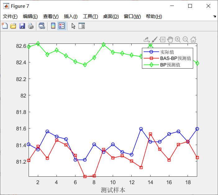
figure
plot(1:length(output_test), output_test,'b-o','linewidth',1)
hold on
plot(1:length(ABCBPsim),ABCBPsim,'r-square','linewidth',1)
hold on
plot(1:length(Tsim1),Tsim1,'g-diamond','linewidth',1)
xlabel('Test sample','FontSize',12);
legend('actual value','BAS-BP Estimate','BP Estimate');
axis tight
%% Result evaluation
Result1=CalcPerf(output_test,ABCBPsim);
MSE1=Result1.MSE;
RMSE1=Result1.RMSE;
MAPE1=Result1.Mape;
disp(['BASBP-RMSE = ', num2str(RMSE1)])
disp(['BASBP-MSE = ', num2str(MSE1)])
disp(['BASBP-MAPE = ', num2str(MAPE1)])
Result2=CalcPerf(output_test,Tsim1);
MSE2=Result2.MSE;
RMSE2=Result2.RMSE;
MAPE2=Result2.Mape;
disp(['BP-RMSE = ', num2str(RMSE2)])
disp(['BP-MSE = ', num2str(MSE2)])
disp(['BP-MAPE = ', num2str(MAPE2)])3 simulation results
4 references
[1] Niu Qing, Cao Aimin, Chen Xiaoyi, Zhou Dong. Short term load forecasting based on flower pollination algorithm and BP neural network [J]. Power grid and clean energy, 2020,36 (10): 28-32
[2] Wang Jie. Research and prediction application of neural network parallel optimization based on longicorn whisker search algorithm [D]. Hangzhou University of Electronic Science and technology, 2020